Curve of a Function
We now learn how to represent functions graphically.
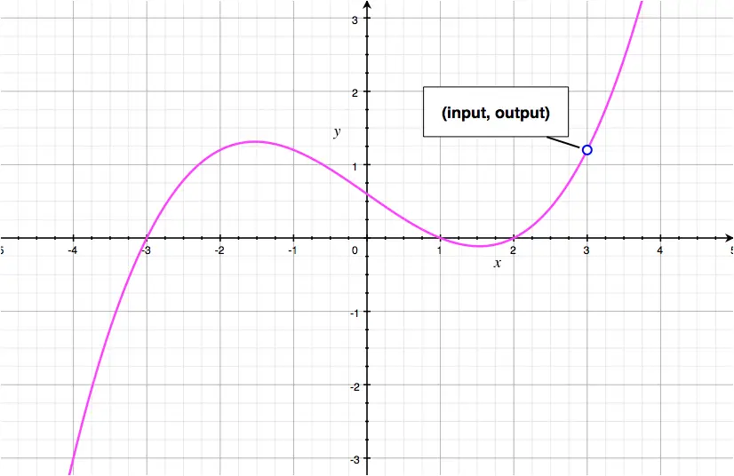
A function \(f(x)\) can be illustrated by its curve on an \(xy\) grid. This allows us to see all of the input/output values of a function with a single curve.
Given a domain, a function's curve is made of an infinite number of connected points.
Each point on the curve has \(x\) and \(y\) coordinates, \(\begin{pmatrix}x,y\end{pmatrix}\) taken as:
- \(x = \text{input value}\)
- \(y = \text{output value}\)
So given a function and its domain it's curve is the collection of all the points with coordinates: \[\begin{pmatrix}\text{input}, \text{output} \end{pmatrix}\] Where each of the input values is an element of the function's domain.
Another way of 'thinking of'/writing this is: \[\begin{pmatrix}x, \ f(x) \end{pmatrix}\]
Since we can't possibly calculate the coordinate's all of the points that make a curve: to draw a function's curve we calculate the coordinates of a few points and draw the curve passing through them (our graphical calculators do the same).
When doing so we usually use a table of values. We learn about these next.
Exam Hint
In exams we'll often be given the table of values that needs to be completed, so the values in the first row (the values of \(x\)) will be given to us.
Table of Values
Given a function \(f(x)\), we can draw its curve (or part of it) using a table of values.
This is typically presented in two rows:
- the first row shows the imput values, those are the \(x\) coordinates of the points along the curve.
- the second row shows the output values, those are the \(y\) coordinates of the points along the curve.
Example 1
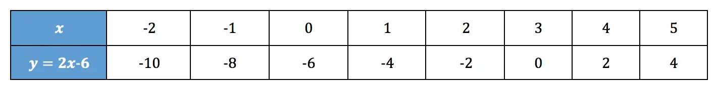
Consider the function \(f(x) = 2x-6\). Its "curve" has equation: \[y = 2x-6\] Suppose we are asked to draw this function's curve, using the following table of values:
Method
We complete the second row by calculating the value of \(y\) for each value of \(x\) shown in the first row.
For \(x = -2\) that would be: \[\begin{aligned}y & = 2\times (-2)-6 \\ & = -4 - 6 \\ y & = -10 \end{aligned}\] Calculating all of the values of \(y\) and completing the table leads to:
Now that we have completed the second row of the table of values we can plot the points.
Each point's coordinates can be read directly from the table. The first couple of points are: \[\begin{pmatrix}-2,-10\end{pmatrix}, \ \begin{pmatrix}-1,-8\end{pmatrix}, \ \dots\] Once we have plotted all of the points:
- look at the trend of the points
- Draw a smooth curve passing through these points.


Example 2
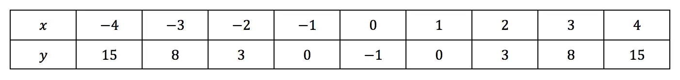
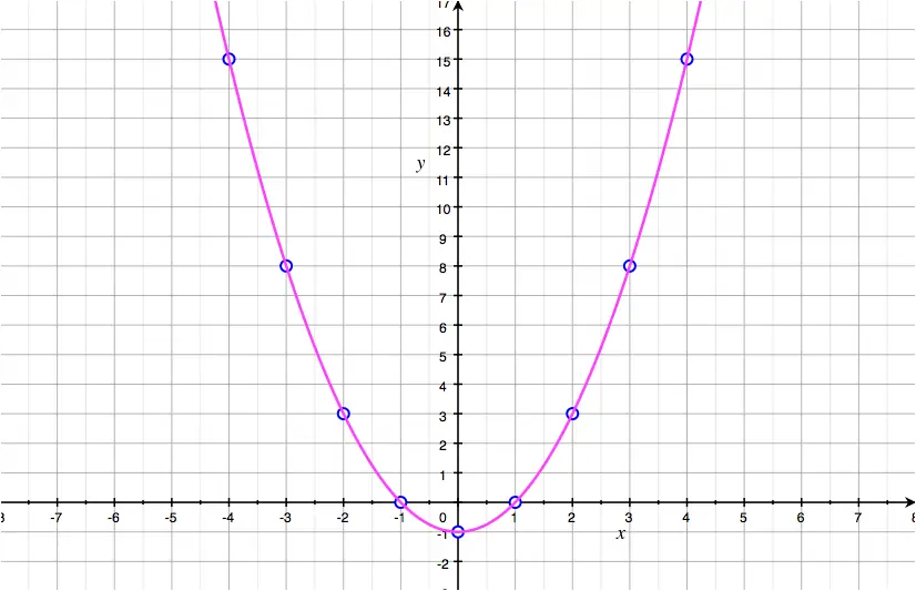
Given the function defined as: \[f(x) = x^2-1\] plot its curve \(y=x^2-1\)
- Copy and complete the following table of values.
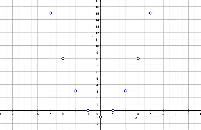
- Plot all the points of the table of values on an \(xy\) grid.
- Draw a smooth curve passing through all of the points.
Tutorial
Exercise
Answers Without Working
Using a Graphical Calculator
To plot functions' curves, we'll often use graphical calculators.
The calculator makes its own table of values (much larger than the ones we did above) and plots enough points for it to appear as a smooth curve on the screen.
The advantage with the calculator is that we can easily find the coordinates of:
- any \(x\)-intercepts (points at which the curve cuts/crosses the \(x\)-axis)
- any minimum, or maximum, point on the curve
The tutorial below shows how to plot a curve with a graphical calculator.
Example
Using a calculator, sketch the curve of \(f(x) = x^2+2x-3\) for \(-5\leq x \leq 3\).
- Label the \(y\)-intercept.
- Label any \(x\)-intercepts (points at which the curve cuts the \(x\)-axis).
- Label any minimum, or maximum point.
Solution
The method for sketching the curve as well as finding each of the points asked for is explained in the following tutorial.