Normal Distributions

Normal distributions are used to model variables that are evenly spread on either side of their mean values. The further a value is from the mean: the less likely that value is to occur.
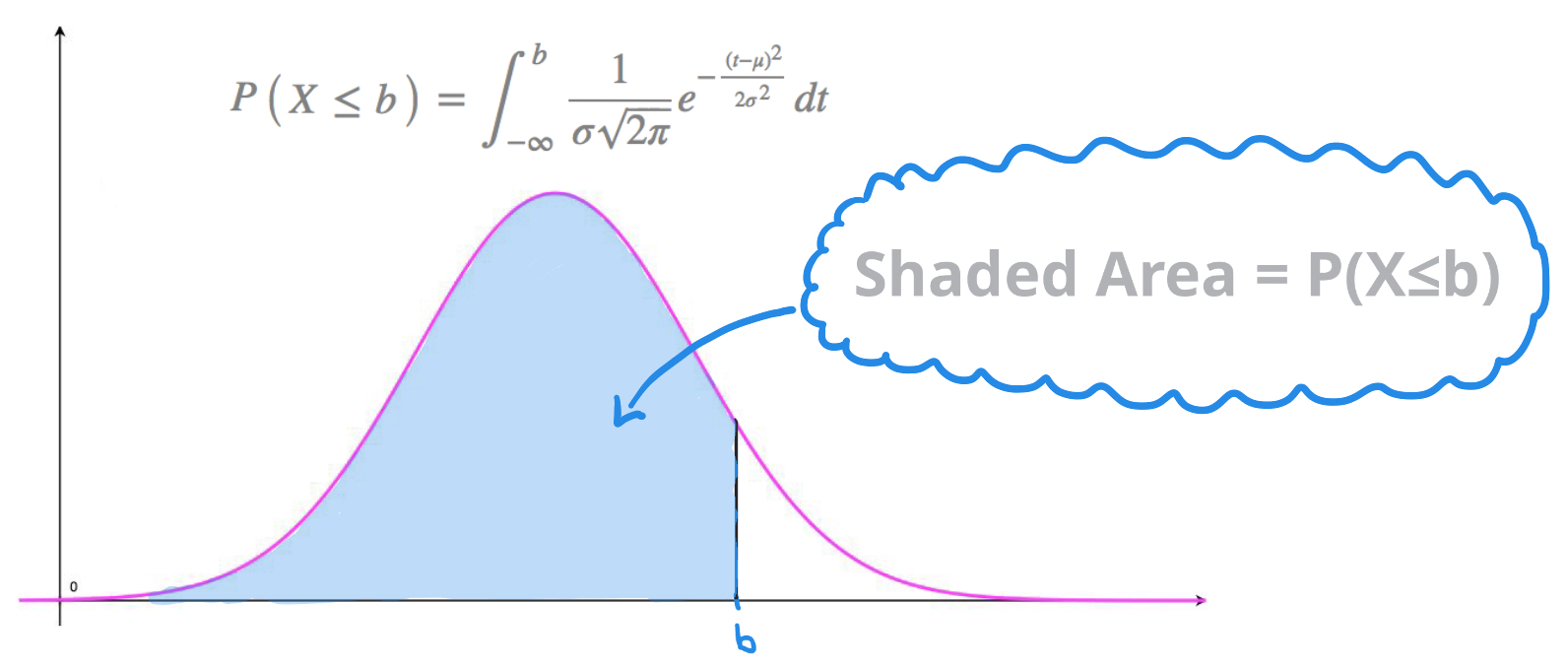
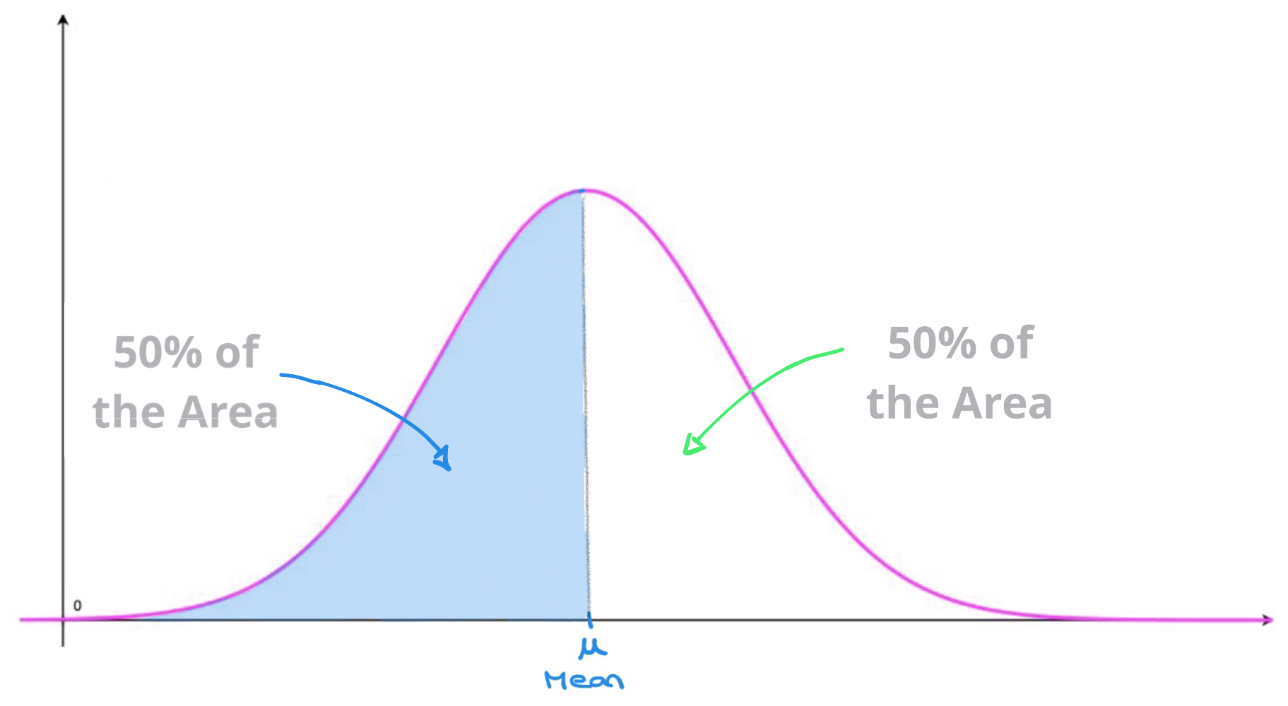
The curve of a normal probability density function appears to be bell-shaped. These curves are often referred to as bell curves.
Bell curves are symmetrical on either side of the mean value \(x=\mu\) so that \(50\%\) of the area enclosed by the curve and the horizontal axis lies on either side of the vertical line of symmetry \(x=\mu\).

An example could be the distribution of the heights in cm of the entire male population of a country. There would be a mean height (say 175cm) and all heights in the population would be evenly distributed on either side of this mean, with a standard deviation of a few cm.
Another example could be the time it takes for each gender to run \(100\)m. There would be a mean value and all other values would be evenly spread on either side of that mean.

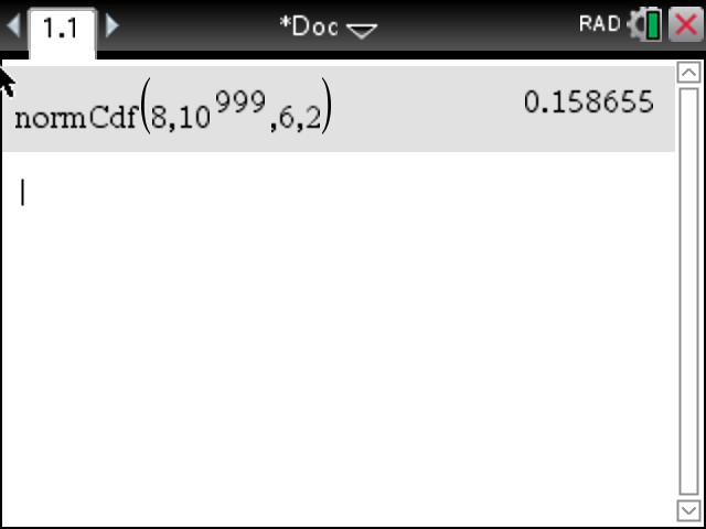
To say that a continuous random variable, \(X\), follows a normal distribution with mean \(\mu \) and variance \(\sigma^2\) we write: \[X \sim N\begin{pmatrix} \mu , \ \sigma^2 \end{pmatrix}\] Remember: \(\text{Variance}=\sigma^2\), where \(\sigma \) is the standard deviation.

Probability Density Function (PDF)

Given a continuous random variable that follows a normal distribution, \(X \sim N\begin{pmatrix} \mu , \ \sigma^2 \end{pmatrix}\), its probability density function, \(f(x)\), is defined as: \[f(x)=\frac{1}{\sigma \sqrt{2 \pi }}e^{- \frac{(x-\mu )^2}{2\sigma^2}}, \quad x\in \mathbb{R}\] Note: we'll rarely need to manipulate this function. In general any work we do with normal distributions is done with a calculator or a computer (that has the normal distribution function built-in to it).

Mean, Median, Mode

Normal distributions are such that mean, median and mode are all equal to eachother. So given a normal distribution we can state: \[\text{mean} = \mu\] \[\text{median} = \mu\] \[\text{mode} = \mu\]

Properties of the Normal PDF

A few properties of this function should always be kept in mind:

the function \(f(x)=\frac{1}{\sigma \sqrt{2 \pi }}e^{- \frac{(x-\mu )^2}{2\sigma^2}}\) always has values greater than, or equal to, \(0\). That's: \[f(x)\geq 0, \quad x\in \mathbb{R}\]
the total area enclosed by the curve and the horizontal axis is equal to \(1\), that's: \[\int_{-\infty }^{+\infty}f(x)dx = 1\]
the bell curve is symmetrical across its mean, \(\mu \). 50% of the area beneath the curve lies on either side of the \(x = \mu \)
The mean, median and mode are all equal to \(\mu \).

Just as with other continuous probability distributions, this function isn't used to calculate probabilities directly.
We calculate probabilities by calculating areas enclosed by the curve and the horizontal axis.
To do this we use the cumulative distribution function.

Cumulative Distribution Function (CDF)

The cumulative density function (cdf), used to find probability \(P\begin{pmatrix}X \leq x \end{pmatrix}\), of a normal distribution is defined as: \[F(x) = \int_{-\infty}^x \frac{1}{\sigma \sqrt{2 \pi }}e^{- \frac{(t-\mu )^2}{2\sigma^2}} dt \] The value of \(F(x)\) is equal to the probability \(P\begin{pmatrix}X\leq x \end{pmatrix}\), that's: \[F(x)=P\begin{pmatrix}X\leq x\end{pmatrix}\] So, we often simply write: \[P\begin{pmatrix}X \leq x \end{pmatrix} = \int_{-\infty}^x \frac{1}{\sigma \sqrt{2 \pi }}e^{- \frac{(t-\mu )^2}{2\sigma^2}} dt \]

Using the cumulative normal function: calculating probabilities

To calculate the probabiliy \(P\begin{pmatrix} X\leq b \end{pmatrix}\), we calculate \(F(b)\), that's the integral: \[P\begin{pmatrix}X \leq b \end{pmatrix} = \int_{-\infty}^b \frac{1}{\sigma \sqrt{2 \pi }}e^{- \frac{(t-\mu )^2}{2\sigma^2}} dt \] This represents the area enclosed beneath the bell-shaped curve and the horizontal axis, from \(- \infty\) up to \(b\).

This is illustrated here:

The shaded area is equal to the probability \(P\begin{pmatrix} X\leq b \end{pmatrix}\).

Calculating such integrals is very tricky.
Luckily for us our calculators have this integral built-in.

Calculator Technique

and all we have to enter is:

the lower bound,
the upper bound,
the mean \(\mu \),
the standard deviation, \(\sigma \).

On the TI-NSpire CX it is the normCDF function.

Tutorial: TI NSpire CX

Example

A random variable \(X\) follows a normal distribution with mean \(\mu = 6\) and standard deviation \(\sigma = 2\).
Find each of the following probabilities:

\(P\begin{pmatrix}X\leq 3\end{pmatrix}\)
\(P \begin{pmatrix} X>8 \end{pmatrix} \)
\(P \begin{pmatrix} 3 < X < 7 \end{pmatrix} \)

We answer each of these in turn.

To find \(P\begin{pmatrix}X\leq 3\end{pmatrix}\) we need to calculate the integral: \[P\begin{pmatrix}X \leq 3 \end{pmatrix} = \int_{-\infty }^3 \frac{1}{2 \sqrt{2 \pi }}e^{- \frac{(x-6 )^2}{2\times 2^2}} x \] That's: \[P\begin{pmatrix}X \leq3 \end{pmatrix} = \int_{-\infty }^3 \frac{1}{2 \sqrt{2 \pi }}e^{- \frac{(x-6 )^2}{8}} x \] This corresponds to the shaded area beneath the pdf curve, shown here:

To find \(P\begin{pmatrix}X>8\end{pmatrix}\) we need to calculate the integral: \[P\begin{pmatrix}X >8 \end{pmatrix} = \int_8^{+\infty } \frac{1}{2 \sqrt{2 \pi }}e^{- \frac{(x-6 )^2}{2\times 2^2}} x \] That's: \[P\begin{pmatrix}X >8 \end{pmatrix} = \int_8^{+\infty } \frac{1}{2 \sqrt{2 \pi }}e^{- \frac{(x-6 )^2}{8}} x \] This corresponds to the area beneath the curve, as shown here:

Using the normal cdf function on the TI NSpire-CX to calculate this integral, we enter the following:

Note: we enter \(10^{999}\) as the upper bound as we cannot enter \(+\infty \).

Pressing "ok" leads us to the following result:

So \(P\begin{pmatrix}X>8\end{pmatrix} = 0.158655\).

Rounding this result to 3 significant figures, that's: \(P\begin{pmatrix}X>8\end{pmatrix} = 0.159\).

Important Results the Normal CDF

Just as for other continuous probability distributions: \[P\begin{pmatrix}X \leq k \end{pmatrix} = P\begin{pmatrix}X < k \end{pmatrix}\] \[P\begin{pmatrix}X \geq k \end{pmatrix} = P\begin{pmatrix}X > k \end{pmatrix}\] Consequently: \[\begin{aligned}P\begin{pmatrix}a \leq X \leq b \end{pmatrix} & = P\begin{pmatrix} a < X < b \end{pmatrix} \\ & = P\begin{pmatrix} a \leq X < b \end{pmatrix} \\ & = P\begin{pmatrix} a < X \leq b \end{pmatrix} \end{aligned}\]

Exercise 1

Answer each of the following:

In France, the average male height is 175cm.
It is believed that men's height follows a normal distribution, with standard deviation \(\sigma = 5\).
1. Find the probability that a French man measures less than \(177\)cm.
2. Find the probability that a French man measures more than \(180cm\).
3. Find the probability that a French man measures between \(170\)cm and \(180\)cm.
A high school athletics club has a team of sprinters. The time taken to run the \(100\)m sprint follows a normal distribution with a mean time of \(13\) seconds and a standard deviation of \(2\) seconds.
1. Find the probability that a runner takes less than \(11\) seconds to run the \(100\)m.
2. Find the probability that a runner takes less than \(10\) seconds to run the \(100\)m.
3. Students who are able to run the \(100\)m in \(11\) to \(12\) seconds are considered excellent.
  Find the probability that the time taken to run \(100\)m between \(11\) and \(12\) seconds.

RadfordMathematics.com

Online Mathematics Book