IB Mathematics: Analysis and Approaches HL — Topic 4
Discrete random variables
Probability tables, expectation and variance.
Learning goal
Read probability distributions, calculate mean and spread, transform outcomes and analyse fair games.
Syllabus link
AHL 4.14 The discrete component: variance, standard deviation, fair games and linear transformations. SL 4.7 foundations are reviewed first.
Big idea
Each possible value carries a probability. These probabilities are the weights used to calculate averages.
Key relationship
\(\Var(X)=\E(X^2)-[\E(X)]^2\)
Standard deviation is the square root of variance.
What is a discrete random variable?
A random variable assigns a numerical value to the outcome of a random experiment. It is discrete when its possible values can be listed, either in a finite list or a list that continues indefinitely, such as \(0,1,2,\ldots\). Values may be negative or non-integer; they need not be equally likely. This lesson uses finite distributions.
Capital \(X\) names the random variable; lower-case \(x\) denotes a possible value. The notation \(\Prob(X=x)\) means the probability that \(X\) takes the value \(x\). A probability distribution lists every possible value and its probability.
Worked example 1 — From outcomes to numerical values
Two fair coins are tossed independently. Let \(X\) be the number of heads in the two tosses. Find the probability distribution of \(X\).
Solution
Write H for heads and T for tails. The equally likely outcomes are TT, TH, HT and HH, each with probability \(\frac14\). Their values of \(X\) are 0, 1, 1 and 2.
| \(x\) | \(0\) | \(1\) | \(2\) |
|---|---|---|---|
| \(\Prob(X=x)\) | \(\frac14\) | \(\frac12\) | \(\frac14\) |
Thus \(\Prob(X=1)=\frac12\): two of the four equally likely outcomes produce one head. The three possible values are not equally likely.
Before you start: basic probability, fractions and algebra. Summation notation is explained in section 2. Give exact values unless an approximation is requested.
Read and check a probability distribution
A probability distribution must account for every possible value of \(X\) and give the probability of each value. Before using a proposed distribution, check that it satisfies both rules below.
Suppose there are \(n\) distinct values, labelled \(x_1,x_2,\ldots,x_n\). Write \(p_i=\Prob(X=x_i)\) for the probability attached to the \(i\)th value. For example, in the coin table in example 1, \(x_2=1\) and \(p_2=\frac12\).
Two conditions for a valid discrete probability distribution
1. Every probability must lie between 0 and 1, inclusive. \[\boxed{0\leq p_i\leq1\quad\mathrm{for\ every}i}.\] A probability of 0 means impossible; a probability of 1 means certain. Negative probabilities or probabilities greater than 1 are not allowed.
2. The probabilities of all the distinct values must add to 1. \[\boxed{p_1+p_2+\cdots+p_n=\sum_{i=1}^{n}p_i=1}.\] On each trial, \(X\) must take one of the listed values, and it cannot take two different values at once. The total probability is therefore \(100\%=1\).
The symbol \(\sum\) means “add”: \(i\) runs from 1 to \(n\), so include each probability once. We are adding the probabilities, not the values of \(X\).
A distribution can also be given by a probability mass function, \(p(x)=\Prob(X=x)\), together with its allowed values. Check the same two conditions for the probabilities it produces.
Worked example 2 — Find a normalising constant
Let \(X\) be the number of tokens in a randomly selected envelope, with \[\begin{gathered}\Prob(X=x)=k(x+1),\\x\in\{1,2,3\}.\end{gathered}\] and probability zero for all other values. Find \(k\) and check that the distribution is valid.
Solution
The normalising constant \(k\) makes the probabilities add to 1: \[\begin{aligned}k(1+1)&+k(2+1)\\&+k(3+1)=1,\\9k&=1,\\k&=\frac19.\end{aligned}\]
| \(x\) | \(1\) | \(2\) | \(3\) |
|---|---|---|---|
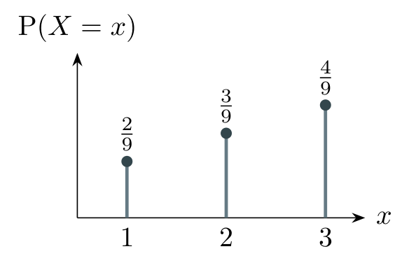
| \(\Prob(X=x)\) | \(\frac29\) | \(\frac39\) | \(\frac49\) |
Each entry lies between 0 and 1; their sum is \(\frac29+\frac39+\frac49=1\). Both conditions hold.
The stem at each \(x\) has height \(\Prob(X=x)\). Values outside the table have probability zero.
Quick check A
For this distribution, find \(\Prob(X=2)\) and \(\Prob(X=2.5)\).
Show solution
Solution
\[\begin{aligned} \Prob(X=2)&=\frac39=\boxed{\frac13},\\ \Prob(X=2.5)&=\boxed0. \end{aligned}\] The value 2.5 is not one of the allowed values 1, 2 and 3.
Related tutorial: Distribution tables and bar charts
SL 4.7 prerequisite revision. Read and represent a discrete probability distribution.
Calculate probabilities from a distribution
An event is a condition that may or may not be satisfied by the outcome. For example, \(X\geq1\) is the event that the value of \(X\) is at least 1.
Choose the values that satisfy the condition
Add the relevant probabilities. List the possible values of \(X\) that satisfy the condition, then add their probabilities. Different values of \(X\) cannot occur together on the same trial.
Use the complement when it is shorter. The complement of an event is the event that it does not happen. Their probabilities add to 1. For any fixed number \(k\), \[\Prob(X\leq k)=1-\Prob(X>k).\] The complement of “at most \(k\)” is “greater than \(k\)”; the value \(k\) belongs to only one side.
Worked example 3 — Inequalities and endpoints
Let \(X\) be the change in a player’s score, in points, after one round:
| \(x\) | \(-2\) | \(0\) | \(1\) | \(3\) |
|---|---|---|---|---|
| \(\Prob(X=x)\) | \(\frac1{10}\) | \(\frac2{10}\) | \(\frac4{10}\) | \(\frac3{10}\) |
Find:
\(\Prob(X>1)\);
\(\Prob(X\geq1)\);
\(\Prob(X\leq0)\), using the complement.
Solution
Only the value 3 is greater than 1: \[\begin{aligned}\Prob(X>1)&=\Prob(X=3)\\&=\boxed{\frac3{10}}.\end{aligned}\]
Both 1 and 3 are at least 1: \[\Prob(X\geq1)=\frac4{10}+\frac3{10}=\boxed{\frac7{10}}.\]
The complement of \(X\leq0\) is \(X>0\). The positive values in this table are 1 and 3: \[\begin{aligned}\Prob(X\leq0)&=1-\Prob(X>0)\\&=1-\left(\frac4{10}+\frac3{10}\right)\\&=\boxed{\frac3{10}}.\end{aligned}\] Here \(\Prob(X>0)=\Prob(X\geq1)\) because there are no possible values between 0 and 1.
Endpoints matter for a discrete random variable
Here \(\Prob(X>1)\ne\Prob(X\geq1)\) because \(\Prob(X=1)=\frac4{10}\). Including an endpoint can change the probability.
Quick check B
Using the same table, find \(\Prob(-1<X\leq3)\).
Show solution
Solution
The values satisfying \(-1<X\leq3\) are 0, 1 and 3: \[\begin{aligned}\Prob(-1<X\leq3)&=\frac2{10}\\&\quad{}+\frac4{10}\\&\quad{}+\frac3{10}\\&=\boxed{\frac9{10}}.\end{aligned}\]
Conditional probabilities: use the given information
Sometimes we know that an event has happened before calculating another probability. This information restricts the outcomes we consider.
What does “given that” mean?
\(\Prob(A\mid B)\) means the probability that event \(A\) happens, given that event \(B\) has happened. The vertical bar \(\mid\) is read as “given that”.
The intersection \(A\cap B\) is the event that both \(A\) and \(B\) happen. Provided \(\Prob(B)>0\), \[\boxed{\Prob(A\mid B)=\frac{\Prob(A\cap B)}{\Prob(B)}}.\] The denominator is the probability of the given condition. The numerator is the probability of satisfying both requirements.
Worked example 4 — A probability after restricting the outcomes
Use the score-change distribution from example 3:
| \(x\) | \(-2\) | \(0\) | \(1\) | \(3\) |
|---|---|---|---|---|
| \(\Prob(X=x)\) | \(\frac1{10}\) | \(\frac2{10}\) | \(\frac4{10}\) | \(\frac3{10}\) |
Given that the player’s score did not decrease, find the probability that it increased by at least 1 point. In symbols, find \(\Prob(X\geq1\mid X\geq0)\).
Solution
Identify the condition. We are told that \(X\geq0\), so the remaining values are 0, 1 and 3. Their total probability is \[\begin{aligned}\Prob(X\geq0)&=\frac2{10}\\&\quad{}+\frac4{10}\\&\quad{}+\frac3{10}\\&=\frac9{10}.\end{aligned}\] Identify the favourable values within that condition. The values 1 and 3 satisfy both \(X\geq1\) and \(X\geq0\): \[\begin{gathered}\Prob\bigl((X\geq1)\cap(X\geq0)\bigr)\\=\frac4{10}+\frac3{10}\\=\frac7{10}.\end{gathered}\] Divide by the probability of the condition: \[\Prob(X\geq1\mid X\geq0)=\frac{7/10}{9/10}=\boxed{\frac79}.\] The probability is \(\frac79\) among trials in which the score did not decrease.
Use the probability weights
The three remaining values 0, 1 and 3 are not equally likely. Two of them are favourable, but this does not make the answer \(\frac23\). Their probability weights must be used.
Quick check C
Using the same distribution, find \(\Prob(X=3\mid X>0)\).
Show solution
Solution
Given \(X>0\), only 1 and 3 remain, with total probability \(\frac7{10}\): \[\Prob(X=3\mid X>0)=\frac{3/10}{7/10}=\boxed{\frac37}.\]
Expected value: an average weighted by probability
What average value would we expect over many repetitions of the experiment?
Mean or expected value
\[\boxed{\mu=\E(X)=\sum_{i=1}^{n}x_ip_i}.\] Multiply each possible value by its probability, then add. The symbol \(\mu\) (“mu”) denotes the mean. It describes the long-run average under the same model; it need not be a possible outcome.
Worked example 5 — A prize-envelope model
Let \(X\) be the token count in a randomly selected envelope from a new supply:
| \(x\) | \(0\) | \(2\) | \(5\) |
|---|---|---|---|
| \(\Prob(X=x)\) | \(\frac15\) | \(\frac12\) | \(\frac3{10}\) |
Find and interpret the expected number of tokens.
Solution
\[\begin{aligned}\E(X)&=0\left(\frac15\right)\\&\quad{}+2\left(\frac12\right)\\&\quad{}+5\left(\frac3{10}\right)\\&=\boxed{\frac52\,\mathrm{tokens}}.\end{aligned}\] Over 1000 independent selections, counts of about 200, 500 and 300 would give an average of \[\begin{gathered}\frac{200(0)+500(2)+300(5)}{1000}\\=2.5\,\mathrm{tokens}.\end{gathered}\] The actual counts fluctuate. No individual envelope contains 2.5 tokens.
Worked example 6 — A mean can determine missing probabilities
The possible scores \(X\) in a game are 0, 1 and 3 points, with probabilities \(a\), \(b\) and \(\frac14\). Given that \(\E(X)=\frac54\), find \(a\) and \(b\).
Solution
Use two facts: total probability is 1, and the mean is \(\frac54\): \[\begin{aligned} a+b+\frac14&=1,\\ 0a+1b+3\left(\frac14\right)&=\frac54. \end{aligned}\] The mean equation gives \(b=\frac54-\frac34=\frac12\). Then \(a=1-\frac14-\frac12=\frac14\).
The probabilities \(\frac14,\frac12,\frac14\) lie between 0 and 1 and sum to 1.
The mean is not necessarily the most likely value
In example 5, the most likely count is 2 tokens, while the mean is 2.5 tokens. Also, \((0+2+5)/3\) ignores the unequal probabilities and gives the wrong mean.
Quick check D
Let \(W\) take values \(0,2,4\) with probabilities \(\frac12,\frac14,\frac14\). Find \(\E(W)\). Is this mean a possible value of \(W\)?
Show solution
Solution
\[\begin{aligned}\E(W)&=0(\tfrac12)\\&\quad{}+2(\tfrac14)\\&\quad{}+4(\tfrac14)\\&=\boxed{\frac32}.\end{aligned}\] The mean 1.5 is not a possible value of \(W\); the possible values are 0, 2 and 4.
Related tutorial: Mean and mode of a discrete random variable
Mean: SL 4.7 revision, used in AHL 4.14. The mode is the value (or values) with greatest probability.
Variance and standard deviation
The mean describes the centre. Variance measures spread around that mean. The standard deviation is the square root of the variance. We write \(\sigma\) (“sigma”) for the standard deviation, so \(\sigma^2=\Var(X)\).
Four steps: mean, squared values, variance, standard deviation
Find the mean: \(\displaystyle \mu=\E(X)=\sum x_ip_i\).
Find \(\displaystyle \E(X^2)=\sum x_i^2p_i\): square each value, multiply by its original probability, then add. This is also called the second moment (about zero).
Find the variance: \(\boxed{\Var(X)=\E(X^2)-[\E(X)]^2}\).
Find the standard deviation: \(\boxed{\sigma=\sqrt{\Var(X)}}\).
Variance has squared units; standard deviation has the same units as \(X\).
Worked example 7 — Spread of the token count
Use the envelope distribution from example 5: \(X=0,2,5\) tokens with probabilities \(\frac15,\frac12,\frac3{10}\). We already know \(\E(X)=\frac52\) tokens. Find:
\(\E(X^2)\);
the variance of \(X\);
the standard deviation of \(X\).
Solution
Square each value and multiply by its probability: \[\begin{aligned}\E(X^2)&=0^2\left(\frac15\right)\\&\quad{}+2^2\left(\frac12\right)\\&\quad{}+5^2\left(\frac3{10}\right)\\&=\frac{19}{2}\,\mathrm{tokens}^2.\end{aligned}\]
Subtract the square of the mean: \[\begin{aligned}\Var(X)&=\frac{19}{2}-\left(\frac52\right)^2\\&=\boxed{\frac{13}{4}\,\mathrm{tokens}^2}.\end{aligned}\]
Take the square root of the variance: \[\begin{aligned}\sigma&=\sqrt{\frac{13}{4}}\\&=\boxed{\frac{\sqrt{13}}2\,\mathrm{tokens}}\\&\approx1.80\,\mathrm{tokens}.\end{aligned}\]
A brief terminology note
Variance is the mean squared deviation from the mean: the probability-weighted average of \((x-\mu)^2\). Thus \(\Var(X)=\sum(x_i-\mu)^2p_i\geq0\). The equivalent formula \(\E(X^2)-[\E(X)]^2\) is usually shorter for calculations.
Keep the order clear: \(\E(X^2)\) means “square, then average”; \([\E(X)]^2\) means “average, then square”.
Quick check E
For \(W\) in quick check D, we have \(\E(W)=\frac32\). Find \(\E(W^2)\), \(\Var(W)\) and the standard deviation.
Show solution
Solution
\[\begin{aligned}\E(W^2)&=0^2(\tfrac12)\\&\quad{}+2^2(\tfrac14)\\&\quad{}+4^2(\tfrac14)\\&=\boxed5,\\\Var(W)&=5-(\tfrac32)^2\\&=\boxed{\frac{11}{4}},\\\sigma_W&=\sqrt{\frac{11}{4}}\\&=\boxed{\frac{\sqrt{11}}2}.\end{aligned}\]
Related tutorial: Variance and standard deviation
AHL 4.14. Calculate the second moment, subtract the square of the mean, then take the square root.
Interpret spread and find unknown probabilities
Two distributions can have the same mean but different spreads. A smaller variance means that values are more concentrated around the mean. A subscript identifies the variable: \(\sigma_A\) is the standard deviation of \(A\), and \(\sigma_B\) is that of \(B\).
Worked example 8 — Same mean, different spread
Two machines label packs containing two items. Let \(A\) and \(B\) be the number of unlabelled items in a pack from machines A and B, respectively.
| \(x\) | 0 | 1 | 2 |
|---|---|---|---|
| \(\Prob(A=x)\) | 0.1 | 0.8 | 0.1 |
| \(\Prob(B=x)\) | 0.4 | 0.2 | 0.4 |
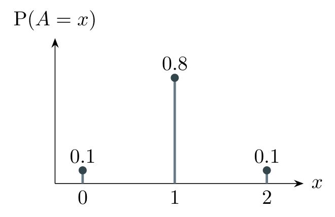
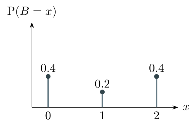
Compare the means, variances and standard deviations of \(A\) and \(B\).
Solution
\[\begin{aligned}\E(A)&=0(0.1)\\&\quad{}+1(0.8)\\&\quad{}+2(0.1)\\&=1,\\\E(B)&=0(0.4)\\&\quad{}+1(0.2)\\&\quad{}+2(0.4)\\&=1.\end{aligned}\] Using \(\Var(X)=\E(X^2)-[\E(X)]^2\), \[\begin{aligned}\Var(A)&=0^2(0.1)\\&\quad{}+1^2(0.8)\\&\quad{}+2^2(0.1)\\&\quad{}-1^2\\&=0.2,\\\Var(B)&=0^2(0.4)\\&\quad{}+1^2(0.2)\\&\quad{}+2^2(0.4)\\&\quad{}-1^2\\&=0.8.\end{aligned}\] \[\begin{aligned} \sigma_A&=\sqrt{0.2}\approx0.447\,\mathrm{items},\\ \sigma_B&=\sqrt{0.8}\approx0.894\,\mathrm{items}. \end{aligned}\]
B has four times the variance of A, but twice its standard deviation: \(\sqrt{0.8}=\sqrt{4\times0.2}=2\sqrt{0.2}\). Both means are 1 item; B is less consistent.
Quick check F
Why must \(\E(X^2)\geq[\E(X)]^2\)? What would a variance of zero mean?
Show solution
Solution
\(\E(X^2)-[\E(X)]^2\) is the variance, which is non-negative. Zero variance means there is no spread: \(X\) equals one constant with probability 1.
Use variance to find an unknown probability
When a distribution contains an unknown parameter, its probabilities must still be valid. Find the allowed range first, then use any given mean or variance to form an equation.
Worked example 9 — An unknown probability from a variance
A discrete score \(X\) takes values 0, 1 and 2 with probabilities \(2p\), \(1-3p\) and \(p\).
Find the range of \(p\) for which this is a valid probability distribution.
Given \(\Var(X)=\frac{14}{25}\), find \(p\) and the probability distribution of \(X\).
Solution
The total is \(2p+(1-3p)+p=1\) for every \(p\). The probabilities must be non-negative: \[\begin{aligned} p\geq0&\quad\Longrightarrow\quad 2p\geq0,\\ 1-3p\geq0&\quad\Longrightarrow\quad p\leq\frac13. \end{aligned}\] Therefore \(\boxed{0\leq p\leq\frac13}\). These probabilities sum to 1, so non-negativity also ensures that each is at most 1.
Calculate the mean and the expected value of \(X^2\): \[\begin{aligned}\E(X)&=0(2p)\\&\quad{}+1(1-3p)\\&\quad{}+2p\\&=1-p,\\\E(X^2)&=0^2(2p)\\&\quad{}+1^2(1-3p)\\&\quad{}+2^2p\\&=1+p.\end{aligned}\] Use the given variance: \[\begin{gathered}\frac{14}{25}=1+p-(1-p)^2,\\\frac{14}{25}=3p-p^2,\\25p^2-75p+14=0,\\ (5p-1)(5p-14)=0.\end{gathered}\] The roots are \(p=\frac15\) and \(p=\frac{14}{5}\). Only \(\frac15\) lies in the allowed range, so \(\boxed{p=\frac15}\).
\(x\) \(0\) \(1\) \(2\) \(\Prob(X=x)\) \(\frac25\) \(\frac25\) \(\frac15\)
An algebraic solution must also be a valid probability model
Substitute each candidate value into the original probabilities. Reject any value that makes a probability negative or greater than 1.
Linear transformations
A linear transformation defines a new random variable by \(Y=aX+b\), where \(a\) and \(b\) are fixed constants. Apply the same calculation to every possible value of \(X\).
For example, let \(X\) be the envelope token count from example 5. If each token pays 2 euros and every envelope also earns a fixed 3-euro bonus, the payout is \(Y=2X+3\) euros:
| \(x\) | 0 | 2 | 5 |
|---|---|---|---|
| \(y=2x+3\) | 3 | 7 | 13 |
| Probability | \(\frac15\) | \(\frac12\) | \(\frac3{10}\) |
Here each new value keeps the probability of its original value. For example, a payout of 7 euros occurs exactly when the envelope contains 2 tokens, so its probability is \(\frac12\).
How the mean and spread change
\[\begin{aligned} \E(Y)&=a\E(X)+b,\\ \Var(Y)&=a^2\Var(X),\\ \sigma_Y&=|a|\sigma_X. \end{aligned}\] The subscripts identify the random variable: \(\sigma_X\) is the standard deviation of \(X\), and \(\sigma_Y\) is that of \(Y\).
Adding \(b\) shifts every value and the mean equally. Multiplying by \(a\) scales distances from the mean by \(|a|\); the absolute value makes the scale factor non-negative.
Worked example 10 — Convert a token count to a payout
For the payout \(Y=2X+3\) above, we already know \(\E(X)=\frac52\) and \(\Var(X)=\frac{13}{4}\). Find:
the mean payout;
the variance of the payout;
the standard deviation of the payout.
Solution
\(\E(Y)=2(\frac52)+3=\boxed{8\,\mathrm{euros}}\).
\(\Var(Y)=2^2(\frac{13}{4})=\boxed{13\,\mathrm{euros}^2}\).
\(\sigma_Y=\sqrt{13}=\boxed{\sqrt{13}\,\mathrm{euros}}\).
Check the mean using the transformed distribution: \[\begin{aligned}&3\left(\frac15\right)+7\left(\frac12\right)\\&\quad+13\left(\frac3{10}\right)\\&=8\,\mathrm{euros}.\end{aligned}\]
Why does adding \(b\) not change the variance? If \(\mu=\E(X)\), then \[\begin{aligned}Y-\E(Y)&=aX\\&\quad{}+b\\&\quad{}-(a\mu+b)\\&=a(X-\mu).\end{aligned}\] The shift cancels. Distances scale by \(|a|\), so squared distances scale by \(a^2\).
Linear transformations: negative and unknown constants
Worked example 11 — A negative multiplier
For the same envelope count, define a score \(Z=10-2X\) points. We have \(\E(X)=\frac52\) and \(\Var(X)=\frac{13}{4}\). Find:
\(\E(Z)\);
\(\Var(Z)\);
the standard deviation of \(Z\).
Solution
Here \(a=-2\) and \(b=10\).
\[\begin{aligned}\E(Z)&=(-2)(\frac52)+10\\&=\boxed{5\,\mathrm{points}}.\end{aligned}\]
\[\begin{aligned}\Var(Z)&=(-2)^2(\frac{13}{4})\\&=\boxed{13\,\mathrm{points}^2}.\end{aligned}\]
\[\begin{aligned}\sigma_Z&=|-2|(\frac{\sqrt{13}}2)\\&=\boxed{\sqrt{13}\,\mathrm{points}}.\end{aligned}\]
The outcomes \(x=0,2,5\) give \(z=10,6,0\): the negative multiplier reverses their order. Their probabilities remain \(\frac15,\frac12,\frac3{10}\) respectively. If you reorder the values, reorder their probabilities too.
Worked example 12 — Find the constants in a transformation
A random score \(X\) has mean 3 points and variance 4 points\(^2\). The adjusted score \(Y=aX+b\) has mean 8 points and standard deviation 6 points. Given \(a>0\):
find \(a\);
find \(b\).
Solution
First convert the standard deviation to a variance: \(\Var(Y)=6^2=36\). \[36=a^2(4)\quad\Longrightarrow\quad a^2=9.\] The condition \(a>0\) selects \(\boxed{a=3}\).
Use the mean equation: \[\begin{aligned}8&=a(3)+b\\&=3(3)+b\\&\Longrightarrow\boxed{b=-1}.\end{aligned}\]
Use the correct rule
The variance equation determines \(a^2\), so check any information about the sign of \(a\). If \(a=0\), the new variable is the constant \(b\) and has variance zero.
These linear-transformation rules do not apply to \(X^2\): calculate \(\E(X^2)\) using \(\sum x_i^2p_i\).
Quick check G
If \(\E(X)=3\), \(\Var(X)=4\) and \(Y=7-2X\), find the mean, variance and standard deviation of \(Y\).
Show solution
Solution
\[\begin{aligned} \E(Y)&=7-2(3)=\boxed1,\\ \Var(Y)&=(-2)^2(4)=\boxed{16},\\ \sigma_Y&=\sqrt{16}=\boxed4. \end{aligned}\]
Fair games
Define the random quantities and the fixed cost
Let \(R\) be the payout received on one play, \(c\) the fixed entry fee, and \(G=R-c\) the player’s net gain. All are measured in the same currency; \(R\) and \(G\) are random, while \(c\) is a constant. \[\begin{gathered}\mathrm{Fair\ game:}\quad\boxed{\E(G)=0}\\\Longleftrightarrow\\\boxed{c=\E(R)}.\end{gathered}\] Positive expected gain favours the player; negative expected gain is an expected loss. “Fair” refers to the long-run mean, not to any one play.
Worked example 13 — Set a fair fee and interpret a loss
An envelope contains \(X=0,2\) or 5 tokens with probabilities \(\frac15,\frac12,\frac3{10}\). Each token pays 2 euros. Define \(R=2X\) as the payout in euros and \(G=R-c\) as the net gain after paying \(c\) euros. We already know \(\E(X)=\frac52\) and \(\Var(X)=\frac{13}{4}\).
Find the fair entry fee.
If the fee is 6 euros, find and interpret \(\E(G)\).
At the fair fee, find the probability of making a profit.
Find \(\Var(G)\) for any fixed fee \(c\).
Solution
\(\E(R)=2\E(X)=2(\frac52)=5\) euros. A fair game has \(c=\E(R)\), so the fair fee is \(\boxed{5\,\mathrm{euros}}\).
\[\begin{aligned}\E(G)&=\E(R)-6\\&=5-6\\&=\boxed{-1\,\mathrm{euro}}.\end{aligned}\] This is an average loss of 1 euro per play over many repetitions.
At \(c=5\), \(G=2X-5\) takes values \(-5,-1,5\) euros. Only \(X=5\) produces a positive net gain: \[\Prob(G>0)=\Prob(X=5)=\boxed{\frac3{10}}.\]
\[\begin{aligned}\Var(G)&=\Var(2X-c)\\&=2^2\Var(X)\\&=4(\frac{13}{4})\\&=\boxed{13\,\mathrm{euros}^2}.\end{aligned}\] Subtracting a fixed fee does not change the variance.
Fair games: find an unknown prize
Worked example 14 — Find an unknown jackpot
In a different game, let \(R\) be the payout in euros: 0, 10 or \(J\), with probabilities \(\frac45,\frac3{20},\frac1{20}\). The fixed fee is 4 euros; define the net gain \(G=R-4\).
Find the jackpot \(J\) that makes the game fair.
For that jackpot, find the probability that the player makes a profit.
Solution
A fair game has \(\E(G)=0\), so \[\begin{aligned}&0(\tfrac45)+10(\tfrac3{20})\\&\quad+J(\tfrac1{20})-4=0.\end{aligned}\] Thus \(\frac32+\frac{J}{20}=4\), giving \(\boxed{J=50\,\mathrm{euros}}\).
The net gains are \(-4,6,46\) euros. Both payouts of 10 and 50 euros produce a profit: \[\Prob(G>0)=\frac3{20}+\frac1{20}=\boxed{\frac15}.\]
A fair game need not have a 50% chance of profit: occasional large gains can balance frequent losses.
Quick check H
In example 14, the fee rises to 5 euros while the payouts stay the same. Find \(\E(G)\) and \(\Prob(G>0)\).
Show solution
Solution
\[\E(G)=4-5=\boxed{-1\,\mathrm{euro}}.\] Either payout of 10 or 50 euros is still profitable, so \(\Prob(G>0)=\frac3{20}+\frac1{20}=\boxed{\frac15}\).
Choose the calculation and check your result
The essentials
| Valid distribution | \(0\leq p_i\leq1\) and \(\sum p_i=1\) |
|---|---|
| Probability of an event | Add the probabilities of the values in that event. |
| Mean | \(\E(X)=\sum x_ip_i\) |
| Second moment | \(\E(X^2)=\sum x_i^2p_i\) |
| Variance | \(\Var(X)=\E(X^2)-[\E(X)]^2\) |
| Standard deviation | \(\sigma=\sqrt{\Var(X)}\) |
| Fair game | Set \(\E(\mathrm{net\ gain})=0\). |
| Linear transformation | \(\E(aX+b)=a\E(X)+b\); \(\Var(aX+b)=a^2\Var(X)\) |
| Transformed standard deviation | \(\sigma_{aX+b}=|a|\sigma_X\) |
When using a calculator: evaluate the probability-weighted sums using the formulas above. Keep full precision during the calculation and round only your final answer.
Which information should I use?
Unknown probabilities: use total probability 1 and any given mean or variance. Check that the resulting probabilities are valid.
Unknown transformation constants: use the variance or standard deviation to find the magnitude of \(a\), then use the mean to find \(b\). Check the sign of \(a\).
A fair fee or prize: define the player’s net gain and set its expected value to zero.
Final checks before moving on
Probabilities lie between 0 and 1 and sum to 1.
The mean lies between the smallest and largest possible values.
\(\E(X^2)\geq[\E(X)]^2\), so variance is non-negative.
Standard deviation has the units of \(X\); variance has squared units.
Retain exact values or unrounded calculator values until the final answer.
Practice A: build the core skills
All questions can be answered without a calculator. Give exact values and show your probability sums. Try each question first, then expand its solution when you are ready to check your work.
1. Outcomes and a distribution
Three fair coins are tossed independently. Let \(X\) be the number of heads.
Construct the distribution of \(X\).
Find \(\Prob(X\geq2)\).
Find the mean and variance.
Show solution
Solution
The eight equally likely outcomes give 0 heads once, 1 head three times, 2 heads three times and 3 heads once:
\(x\) \(0\) \(1\) \(2\) \(3\) \(\Prob(X=x)\) \(\frac18\) \(\frac38\) \(\frac38\) \(\frac18\) \(\Prob(X\geq2)=\frac38+\frac18=\boxed{\frac12}\).
\[\begin{aligned}\E(X)&=0(\frac18)\\&\quad{}+1(\frac38)\\&\quad{}+2(\frac38)\\&\quad{}+3(\frac18)\\&=\boxed{\frac32}.\end{aligned}\] \[\begin{aligned}\E(X^2)&=0^2(\tfrac18)\\&\quad{}+1^2(\tfrac38)\\&\quad{}+2^2(\tfrac38)\\&\quad{}+3^2(\tfrac18)\\&=3.\end{aligned}\] Hence \(\boxed{\Var(X)=3-(\frac32)^2=\frac34}\).
2. A distribution given by a formula
\(\Prob(X=x)=kx\) for \(x\in\{1,2,3,4\}\), and zero otherwise.
Find \(k\).
Find \(\Prob(X>2)\).
Find \(\Prob(X=4\mid X>2)\).
Find \(\E(X)\) and \(\Var(X)\).
Show solution
Solution
\[\begin{aligned}k+2k+3k+4k&=1\\&\Rightarrow\boxed{k=\frac1{10}}.\end{aligned}\]
\(\Prob(X>2)=\frac3{10}+\frac4{10}=\boxed{\frac7{10}}\).
\[\begin{aligned}\Prob(X=4\mid X>2)&=\frac{4/10}{7/10}\\&=\boxed{\frac47}.\end{aligned}\]
\(\E(X)=\frac{1^2+2^2+3^2+4^2}{10}=\boxed3\). \[\begin{aligned}\E(X^2)&=1^2(\tfrac1{10})\\&\quad{}+2^2(\tfrac2{10})\\&\quad{}+3^2(\tfrac3{10})\\&\quad{}+4^2(\tfrac4{10})\\&=10.\end{aligned}\] Therefore \(\boxed{\Var(X)=10-3^2=1}\).
3. Unknown probabilities
The score change \(X\), in points, has this distribution:
| \(x\) | \(-1\) | \(0\) | \(2\) | \(3\) |
|---|---|---|---|---|
| \(\Prob(X=x)\) | \(a\) | \(\frac15\) | \(\frac3{10}\) | \(b\) |
Given \(\E(X)=\frac{11}{10}\), find:
\(a\) and \(b\);
\(\E(X^2)\) and \(\Var(X)\).
Show solution
Solution
Total probability: \(a+b=\frac12\). The mean gives \(-a+2(\frac3{10})+3b=\frac{11}{10}\), so \(-a+3b=\frac12\). Adding the equations gives \(4b=1\), hence \(\boxed{a=b=\frac14}\).
\[\begin{aligned}\E(X^2)&=(-1)^2(\frac14)\\&\quad{}+0^2(\frac15)\\&\quad{}+2^2(\frac3{10})\\&\quad{}+3^2(\frac14)\\&=\boxed{\frac{37}{10}}\end{aligned}\] points\(^2\). \[\begin{aligned}\Var(X)&=\frac{37}{10}-\left(\frac{11}{10}\right)^2\\&=\frac{249}{100}\,\mathrm{points}^2.\end{aligned}\]
4. A full moment calculation
\(X\) takes the values \(-2,1,4\) with probabilities \(\frac14,\frac12,\frac14\).
Find \(\E(X)\) and \(\E(X^2)\).
Find the variance and standard deviation.
Explain why \(\E(X^2)\ne[\E(X)]^2\).
Show solution
Solution
\[\begin{aligned}\E(X)&=(-2)(\frac14)\\&\quad{}+1(\frac12)\\&\quad{}+4(\frac14)\\&=\boxed1.\end{aligned}\] \[\begin{aligned}\E(X^2)&=(-2)^2(\tfrac14)\\&\quad{}+1^2(\tfrac12)\\&\quad{}+4^2(\tfrac14)\\&=\boxed{\frac{11}{2}}.\end{aligned}\]
Find the variance, then its square root: \[\begin{aligned} \Var(X)&=\frac{11}{2}-1^2=\boxed{\frac92},\\ \sigma&=\sqrt{\frac92}=\boxed{\frac{3\sqrt2}{2}}. \end{aligned}\]
Averaging squared values gives \(\frac{11}{2}\); squaring the average gives 1. Their difference is the non-zero variance.
5. Interpret the answer
Let \(X\) be the number of tasks completed in a short session. Its possible values are \(0,1,2\), with probabilities \(\frac15,\frac12,\frac3{10}\).
Find the mean and standard deviation.
Explain what the mean says about many sessions, even though it is not an integer.
Show solution
Solution
Calculate the mean, then the variance and standard deviation: \[\begin{aligned}\E(X)&=0(\tfrac15)\\&\quad{}+1(\tfrac12)\\&\quad{}+2(\tfrac3{10})\\&=\boxed{\frac{11}{10}\,\mathrm{tasks}},\\\E(X^2)&=0^2(\tfrac15)\\&\quad{}+1^2(\tfrac12)\\&\quad{}+2^2(\tfrac3{10})\\&=\frac{17}{10},\\\Var(X)&=\frac{17}{10}-(\tfrac{11}{10})^2\\&=\frac{49}{100},\\\sigma&=\sqrt{\frac{49}{100}}\\&=\boxed{\frac7{10}\,\mathrm{tasks}}.\end{aligned}\]
Over many sessions under this model, the average count approaches 1.1 tasks per session. An individual session completes 0, 1 or 2 tasks.
Practice B: connect the ideas
6. A negative multiplier
A random score \(X\) has mean 4 and variance 9. Define an adjusted score \(Y=5-2X\).
Find the mean, variance and standard deviation of \(Y\).
Explain why adding 5 does not change the standard deviation.
Show solution
Solution
Apply the transformation rules: \[\begin{aligned} \E(Y)&=5-2(4)=\boxed{-3},\\ \Var(Y)&=(-2)^2(9)=\boxed{36},\\ \sigma_Y&=\sqrt{36}=\boxed6. \end{aligned}\]
Adding 5 shifts every score and the mean by 5, so distances from the mean stay unchanged.
7. Fair entry price and spread
Let \(R\) be the payout in euros from one play of a game. Its values are \(0,5,20\), with probabilities \(\frac12,\frac25,\frac1{10}\). Let \(G=R-c\) be the net gain after paying a fixed fee \(c\) euros.
Find the fair entry fee.
For a fee of 5 euros, find \(\E(G)\) and \(\Prob(G>0)\).
Find \(\Var(R)\) and \(\Var(G)\).
Show solution
Solution
\[\begin{aligned}\E(R)&=0(\frac12)\\&\quad{}+5(\frac25)\\&\quad{}+20(\frac1{10})\\&=4\end{aligned}\] euros. Therefore \(\boxed{c=4\,\mathrm{euros}}\).
At \(c=5\), \[\E(G)=4-5=\boxed{-1\,\mathrm{euro}}.\] A positive gain requires \(R>5\), so \(\Prob(G>0)=\boxed{\frac1{10}}\). A payout of 5 euros only breaks even.
Calculate the second moment and the two variances: \[\begin{aligned}\E(R^2)&=0^2(\tfrac12)\\&\quad{}+5^2(\tfrac25)\\&\quad{}+20^2(\tfrac1{10})\\&=50\,\mathrm{euros}^2,\\\Var(R)&=50-4^2\\&=\boxed{34\,\mathrm{euros}^2},\\\Var(G)&=\Var(R)\\&=\boxed{34\,\mathrm{euros}^2}.\end{aligned}\] Subtracting the fixed fee does not change spread.
8. Find a transformation
The number \(X\) of prizes in a packet is \(0,1,2\) with probabilities \(\frac14,\frac12,\frac14\). A payment \(Y=aX+b\) euros has mean 7 euros and standard deviation \(3\sqrt2\) euros. Given \(a>0\):
find \(\E(X)\) and \(\Var(X)\);
find \(a\) and \(b\);
write the probability distribution of \(Y\).
Show solution
Solution
Calculate the original mean and variance: \[\begin{aligned}\E(X)&=0(\tfrac14)\\&\quad{}+1(\tfrac12)\\&\quad{}+2(\tfrac14)\\&=\boxed1,\\\E(X^2)&=0^2(\tfrac14)\\&\quad{}+1^2(\tfrac12)\\&\quad{}+2^2(\tfrac14)\\&=\frac32,\\\Var(X)&=\frac32-1^2\\&=\boxed{\frac12}.\end{aligned}\]
Use the standard deviation to find \(a\): \[\begin{aligned}\Var(Y)&=(3\sqrt2)^2\\&=18\\&=a^2(\tfrac12).\end{aligned}\] Thus \(a^2=36\); the condition \(a>0\) gives \(\boxed{a=6}\). Then use the mean: \[7=6(1)+b\quad\Longrightarrow\quad\boxed{b=1}.\]
The values of \(Y=6X+1\) are 1, 7 and 13 euros, with probabilities \(\frac14,\frac12,\frac14\) respectively.
9. Find a probability using variance
\(X\) takes the values \(0,1,2\) with probabilities \(p,1-2p,p\).
State the possible range of \(p\).
Find \(\E(X)\) and \(\Var(X)\) in terms of \(p\).
Given \(\Var(X)=\frac35\), find the distribution.
Show solution
Solution
\(p\geq0\) and \(1-2p\geq0\), so \(\boxed{0\leq p\leq\frac12}\).
Calculate the mean and variance: \[\begin{aligned}\E(X)&=0p\\&\quad{}+1(1-2p)\\&\quad{}+2p\\&=\boxed1,\\\E(X^2)&=0^2p\\&\quad{}+1^2(1-2p)\\&\quad{}+2^2p\\&=1+2p,\\\Var(X)&=(1+2p)-1^2\\&=\boxed{2p}.\end{aligned}\]
\(2p=\frac35\Rightarrow p=\frac3{10}\). The probabilities of \(0,1,2\) are \(\boxed{\frac3{10},\frac25,\frac3{10}}\).
10. Compare consistency
Two machines dispense identical 1-gram beads. Let \(A\) and \(B\) be the total bead mass, in grams, in a packet from each machine:
| \(a\) | 1 | 2 | 3 |
|---|---|---|---|
| \(\Prob(A=a)\) | \(\frac1{10}\) | \(\frac8{10}\) | \(\frac1{10}\) |
| \(b\) | 0 | 2 | 4 |
| \(\Prob(B=b)\) | \(\frac14\) | \(\frac12\) | \(\frac14\) |
Find both means and variances.
Which machine gives more consistent masses? Justify your answer.
Show solution
Solution
Calculate each mean and variance: \[\begin{aligned}\E(A)&=1(\tfrac1{10})\\&\quad{}+2(\tfrac8{10})\\&\quad{}+3(\tfrac1{10})\\&=\boxed{2\,\mathrm{g}},\\\E(B)&=0(\tfrac14)\\&\quad{}+2(\tfrac12)\\&\quad{}+4(\tfrac14)\\&=\boxed{2\,\mathrm{g}},\\\E(A^2)&=1^2(\tfrac1{10})\\&\quad{}+2^2(\tfrac8{10})\\&\quad{}+3^2(\tfrac1{10})\\&=\frac{21}{5},\\\Var(A)&=\frac{21}{5}-2^2\\&=\boxed{\frac15\,\mathrm{g}^2},\\\E(B^2)&=0^2(\tfrac14)\\&\quad{}+2^2(\tfrac12)\\&\quad{}+4^2(\tfrac14)\\&=6,\\\Var(B)&=6-2^2\\&=\boxed{2\,\mathrm{g}^2}.\end{aligned}\]
Machine A is more consistent: its masses have smaller variance around the same mean.
Tutorial guide
Watch the embedded videos or follow the YouTube links. All four tutorials are by Radford Mathematics.
Which videos support this syllabus section?
The variance and standard deviation tutorial directly supports AHL 4.14. Distribution tables and expected value are introduced in SL 4.7 and provide the foundations used here. The discrete median tutorial is optional review: AHL 4.14 explicitly specifies median and mode for continuous random variables.
Related tutorial: Distribution tables and bar charts
SL 4.7 prerequisite revision. Use with section 2 to revise probability tables and their graphical representation.
Related tutorial: Mean and mode of a discrete random variable
Mean: SL 4.7 revision, used in AHL 4.14. Use with section 4 . The mode part reviews the value (or values) with greatest probability.
Related tutorial: Variance and standard deviation
AHL 4.14. Use with section 5 to revise \(\E(X^2)\), \(\Var(X)\) and the standard deviation.
Related tutorial: Median of a discrete random variable
Optional review. A separate tutorial on locating a median in a discrete distribution; it is not an additional discrete-median requirement of AHL 4.14.