IB Mathematics: Analysis and Approaches SL/HL — Topic 4 Statistics and Probability
Normal Distributions
From histogram areas to normal probabilities, percentiles and inverse normal.
Learning goal
Interpret a normal model, calculate probabilities and find unknown boundaries using technology.
Syllabus link
AA SL/HL: SL 4.9. Normal distributions, their properties, probability calculations and inverse normal.
Big idea
Choose the interval, shade the region and find its area.
Key relationship
Probability is area under the density curve. The mean \(\mu\) and standard deviation \(\sigma\) determine the normal model.
From histogram areas to a bell curve
Let \(X\) be the height, in cm, of a randomly selected person from a comparable group of adults. Height is a continuous random variable: it can take any value within an interval. The histograms and curve below describe the same ideal normal population.
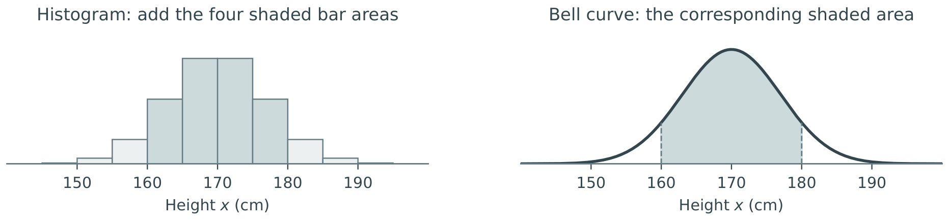
In a relative frequency density histogram, each rectangle’s area represents the percentage of the population in that class interval. The total area represents \(100\%=1\).
Worked example 1 — the same probability, the same shaded region
Question. Find \(\mathrm{P}(160<X<180)\): the probability that the randomly selected person measures between \(160\) and \(180\) cm. Rounded percentages for the four shaded bars are given below.
| Height class (cm) | \(160\leq x<165\) | \(165\leq x<170\) | \(170\leq x<175\) | \(175\leq x<180\) |
|---|---|---|---|---|
| Population (%) | \(16.10\) | \(26.25\) | \(26.25\) | \(16.10\) |
Solution
Add the percentages for the four shaded rectangles: \[(16.10+26.25+26.25+16.10)\%=84.70\%=0.8470.\] Thus \(\mathrm{P}(160<X<180)\approx\boxed{0.847}\): about \(84.7\%\) of the population. The shaded area under the bell curve represents the same probability.
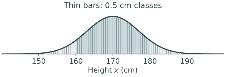
For this ideal normal population, narrowing the classes makes the tops of the rectangles follow the bell curve more closely. We still find a probability by finding the area between the same two heights. The distribution’s shape is a modelling assumption; narrowing the bars does not make data normal.
Which bell curve should we use?
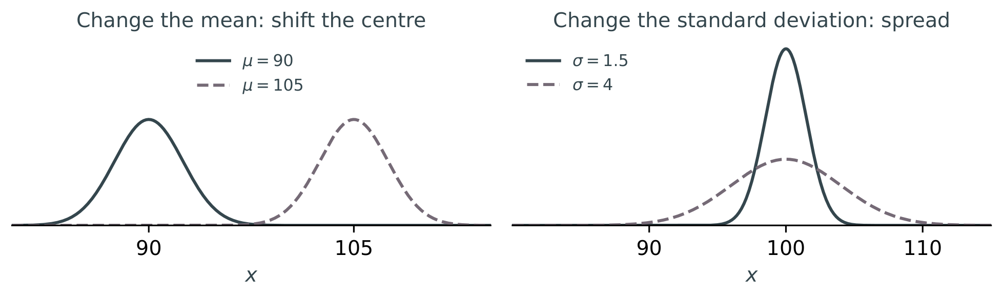
To replace the bell-shaped histogram with a normal model, we need the population’s mean \(\mu\) and standard deviation \(\sigma\). The mean sets the centre; the standard deviation sets the spread. Together, they determine the equation of the normal curve.
For this population, \(\mu=170\) cm and \(\sigma=7\) cm. We now use these values to define its curve. The calculator will find areas under it for us.
Defining the bell curve
A normal distribution, also called a Gaussian distribution, is a continuous probability distribution with a symmetric, bell-shaped density curve. Saying that \(X\) follows a normal distribution means that its probabilities are given by areas under the normal curve defined below.
The equation of the normal probability density function (pdf)
\[f(x)=\frac{1}{\sigma\sqrt{2\pi}}\,e^{-\frac{(x-\mu)^2}{2\sigma^2}}, \qquad x\in\mathbb{R},\quad \sigma>0.\] Here \(\mu\) (“mu”) is the mean and \(\sigma\) (“sigma”) is the standard deviation. Only \(\mu\) and \(\sigma\) vary from one normal bell curve to another. The numbers \(e\) and \(\pi\) are fixed constants; \(x\) runs along the horizontal axis.
You will not need to enter or integrate this formula: it is built into the graphical calculator.
The notation
To say that a continuous random variable \(X\) (such as height, time or weight) follows a normal distribution, we write: \[X\sim\mathrm{N}(\mu,\sigma^2),\qquad \sigma>0.\] The first entry, \(\mu\), is its mean; the second entry, \(\sigma^2\), is its variance, the square of its standard deviation.
Worked example 2 — read the notation
Question. The opening height model is \(X\sim\mathrm{N}(170,49)\). State the mean and standard deviation.
Solution
The mean is \(170\) cm and the standard deviation is \(\sigma=\sqrt{49}=7\) cm. Equivalently, \(X\sim\mathrm{N}(170,7^2)\).
Worked example 3 — understanding the model (optional insight)
Conceptual enrichment: this illustrates the equation; normal probabilities will be found using technology.
Question. Write the probability density function for \(X\sim\mathrm{N}(170,49)\).
Solution
Substitute \(\mu=170\) and \(\sigma=\sqrt{49}=7\) into the formula: \[f(x)=\frac{1}{7\sqrt{2\pi}}\,e^{-\frac{(x-170)^2}{98}}.\] The height \(f(x)\) is a density; probabilities are areas under the curve.
Only the way we calculate the area changes
Remember: probability = area. For the curve \(y=f(x)\) just defined, the shaded area in worked example 1 is the definite integral \[\boxed{\mathrm{P}(160<X<180)=\int_{160}^{180}f(x)\,dx\approx0.847.}\] The histogram adds rectangle areas; the integral gives the corresponding area under the smooth curve. Normal Cdf on the graphical calculator calculates this area for us; we do not integrate by hand.
How changing the parameters changes the curve
Essential properties of the normal curve
The curve is symmetric about \(x=\mu\), and mean = median = mode. The total area is \(1\), with \(0.5\) on each side of \(\mu\). The tails approach the horizontal axis but never meet it.
A single point has zero width and zero area, so \(\mathrm{P}(X=k)=0\). Including an interval endpoint does not change its probability.
The mean sets the centre. Increasing \(\mu\) shifts the curve to the right without changing its shape, provided \(\sigma\) stays the same.
The standard deviation sets the spread. A larger \(\sigma\) gives a wider, lower curve. A smaller \(\sigma\) gives a narrower, taller curve. In both cases, the total area remains \(1\).
Estimate areas without a calculator: the 68–95–99.7 rule
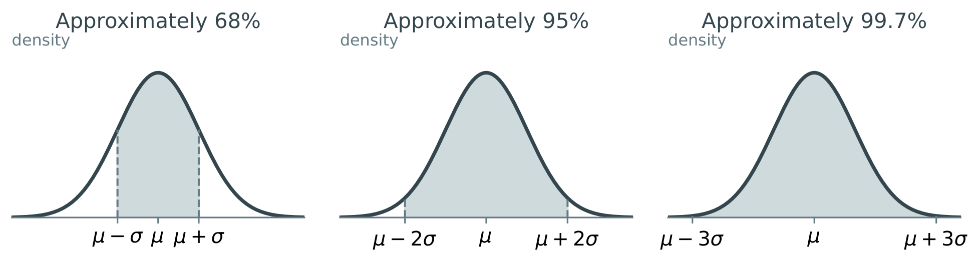
The 68–95–99.7 rule lets us estimate areas without a calculator, using the mean, standard deviation and symmetry. For any normal distribution, approximately: \[\begin{aligned} \mathrm{P}(\mu-\sigma<X<\mu+\sigma)&\approx0.68,\\ \mathrm{P}(\mu-2\sigma<X<\mu+2\sigma)&\approx0.95,\\ \mathrm{P}(\mu-3\sigma<X<\mu+3\sigma)&\approx0.997. \end{aligned}\]
Use symmetry to split the shaded area
An estimate is not a calculator value
Use these rounded percentages when a question asks for an estimate using the rule. For other probability calculations, use the calculator. For example, the area within two standard deviations is about \(95.45\%\), rather than exactly \(95\%\).
Worked example 4 — split the areas using symmetry
Question. \(X\sim\mathrm{N}(88,9^2)\). Without a calculator, use the 68–95–99.7 rule to estimate:
(a) \(\mathrm{P}(X<97)\);
(b) \(\mathrm{P}(X>70)\);
(c) \(\mathrm{P}(79<X<106)\).
Solution
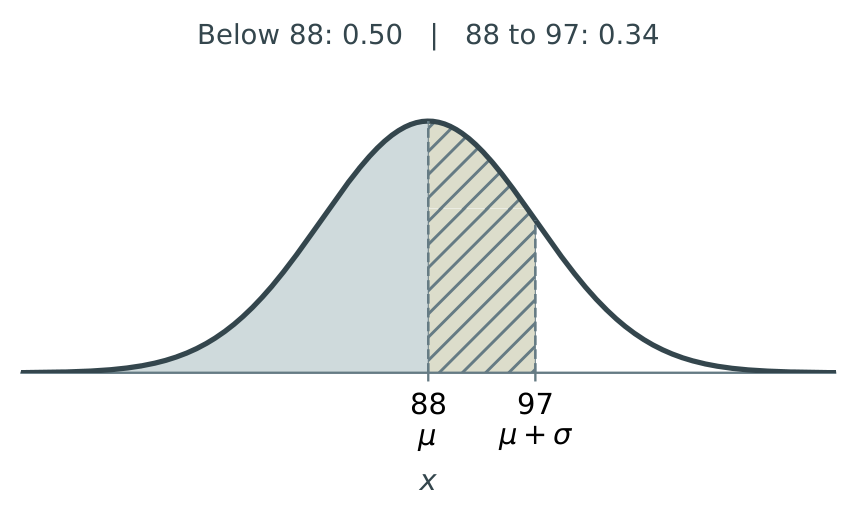
(a) \(97=88+9=\mu+\sigma\).
The area below the mean is \(0.50\). From \(\mu\) to \(\mu+\sigma\), the area is half of \(0.68\), namely \(0.34\). \[\mathrm{P}(X<97)\approx0.50+0.34=\boxed{0.84}.\]
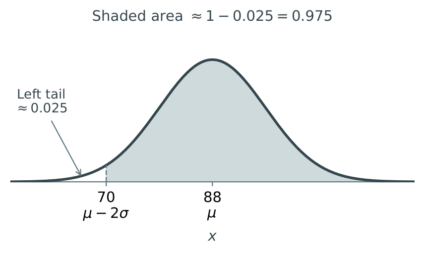
(b) \(70=88-2(9)=\mu-2\sigma\).
The middle \(95\%\) leaves \(5\%\) in the two tails, so each tail has area \(0.05\div2=0.025\). Remove the left tail from \(1\): \[\mathrm{P}(X>70)\approx1-0.025=\boxed{0.975}.\]
(c) \(79=\mu-\sigma\) and \(106=\mu+2\sigma\).
Split the region at the mean, \(88\). Its left part is half of \(0.68\), and its right part is half of \(0.95\): \[\begin{aligned} \mathrm{P}(79<X<106)&\approx0.34+0.475\\ &=\boxed{0.815}. \end{aligned}\]
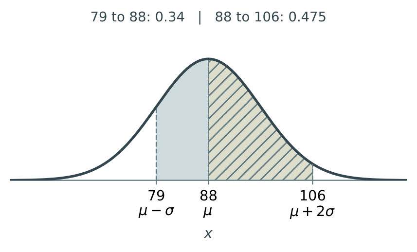
Check each sketch: locate the mean, mark the relevant multiples of \(\sigma\), shade the required region and use the same approximate areas as in the 68–95–99.7 rule.
Use the calculator to find the area
We now replace the table of percentages with the normal model. The routine is unchanged: identify the interval, shade its region and calculate its area. Remember: area = probability.
CDF stands for cumulative distribution function. The calculator’s Normal Cdf command gives the probability between the two bounds you enter.
| Region | Probability statement | Calculator bounds |
|---|---|---|
| Between \(a\) and \(b\) | \(\mathrm{P}(a<X<b)\) | Lower \(a\), upper \(b\) |
| Left of \(k\) | \(\mathrm{P}(X<k)\) | Lower \(-\infty\), upper \(k\) |
| Right of \(k\) | \(\mathrm{P}(X>k)\) | Lower \(k\), upper \(+\infty\) |
TI-Nspire CX: open the calculation Scratchpad.
Choose Menu \(\longrightarrow\) Probability \(\longrightarrow\) Distributions \(\longrightarrow\) Normal Cdf.
Enter the lower bound, upper bound, mean \(\mu\) and standard deviation \(\sigma\). The command is \[\operatorname{normCdf}(\text{lower},\text{upper},\mu,\sigma).\] The initial values \(\mu=0\) and \(\sigma=1\) are defaults. Replace them with the values in your question.
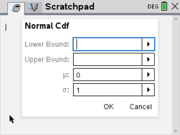
The Normal Cdf input screen.
Worked example 5 — height probabilities on the calculator
Question. The opening height model is \(X\sim\mathrm{N}(170,7^2)\). Use the calculator to find:
(a) \(\mathrm{P}(160<X<180)\);
(b) \(\mathrm{P}(170<X<171)\);
(c) \(\mathrm{P}(X<165)\);
(d) \(\mathrm{P}(X>180)\).
Solution
(a) Between \(160\) and \(180\) cm.
1. Identify and shade the interval. We use the same region as in worked example 1: heights between \(160\) and \(180\) cm.
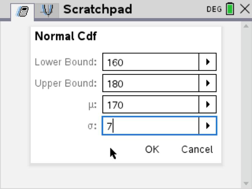
2. Read the model and choose the bounds. The mean is \(\mu=170\) and the standard deviation is \(\sigma=7\). The lower bound is \(160\) and the upper bound is \(180\). \[\mathrm{P}(160<X<180)=\int_{160}^{180}f(x)\,dx =\operatorname{normCdf}(160,180,170,7).\] Enter these four values as shown below, then select OK.
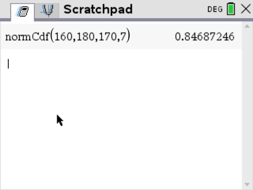
3. Enter the four values, then read the probability. In each pair below, the left screenshot shows the inputs and the right screenshot shows the result.
(a) Between \(160\) and \(180\) cm — calculator result
Interpret the calculator’s answer
The display gives \(0.84687246\), so \[\mathrm{P}(160<X<180)\approx\boxed{0.847}\qquad\text{(3 significant figures).}\] There is approximately an \(84.7\%\) chance that the randomly selected person measures between \(160\) and \(180\) cm. This is the area under the bell curve between those heights.
The four rounded histogram percentages gave \(84.70\%=0.8470\). Both methods give \(0.847\) to three significant figures. The calculator evaluates the area directly; we do not integrate the pdf by hand.
(b) Between \(170\) and \(171\) cm — a narrower interval
Keep \(\mu=170\) and \(\sigma=7\), and change the bounds to \(170\) and \(171\).
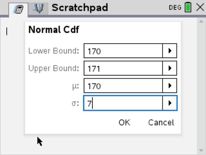
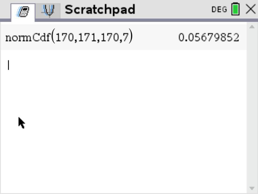
\[\mathrm{P}(170<X<171)=\operatorname{normCdf}(170,171,170,7)\approx\boxed{0.0568}.\] The display gives \(0.05679852\): about \(5.68\%\) of the population. The matching \(1\) cm histogram bar is shown in Appendix A.
Entering \(-\infty\) and \(+\infty\) on the TI-Nspire CX
Press the \(\pi\) key to open the symbols menu, then select \(\infty\). For \(-\infty\), put a minus sign before the symbol.
For the scales in these examples, large bounds such as \(-10^9\) and \(10^9\) (or \(-999999999\) and \(999999999\)) give the same rounded answers. This is the approach used in the tutorial.
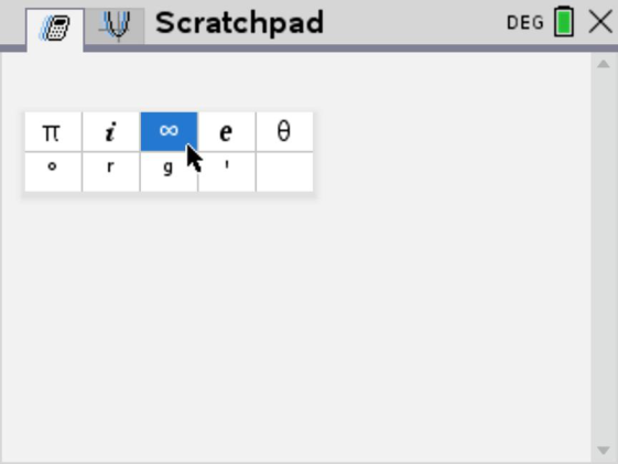
Use infinite bounds for the two tails.
The mean remains \(\mu=170\) and the standard deviation remains \(\sigma=7\). Only the bounds change.
(c) Less than \(165\) cm — a left tail
The left tail extends to \(-\infty\): enter lower bound \(-\infty\) and upper bound \(165\).
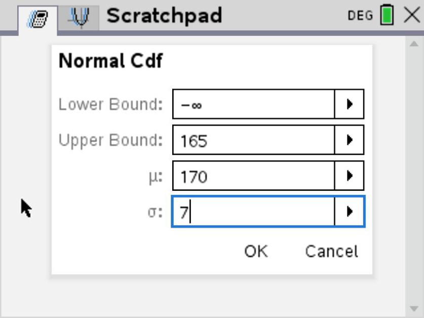
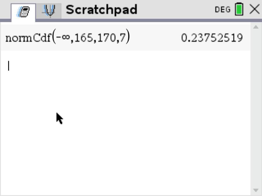
\[\mathrm{P}(X<165)=\operatorname{normCdf}(-\infty,165,170,7)\approx\boxed{0.238}.\] The display gives \(0.23752519\), so approximately \(23.8\%\) of the population measures less than \(165\) cm.
(d) Greater than \(180\) cm — a right tail
The right tail extends to \(+\infty\): enter lower bound \(180\) and upper bound \(\infty\).
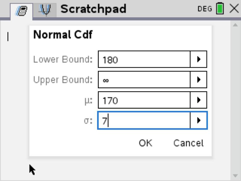
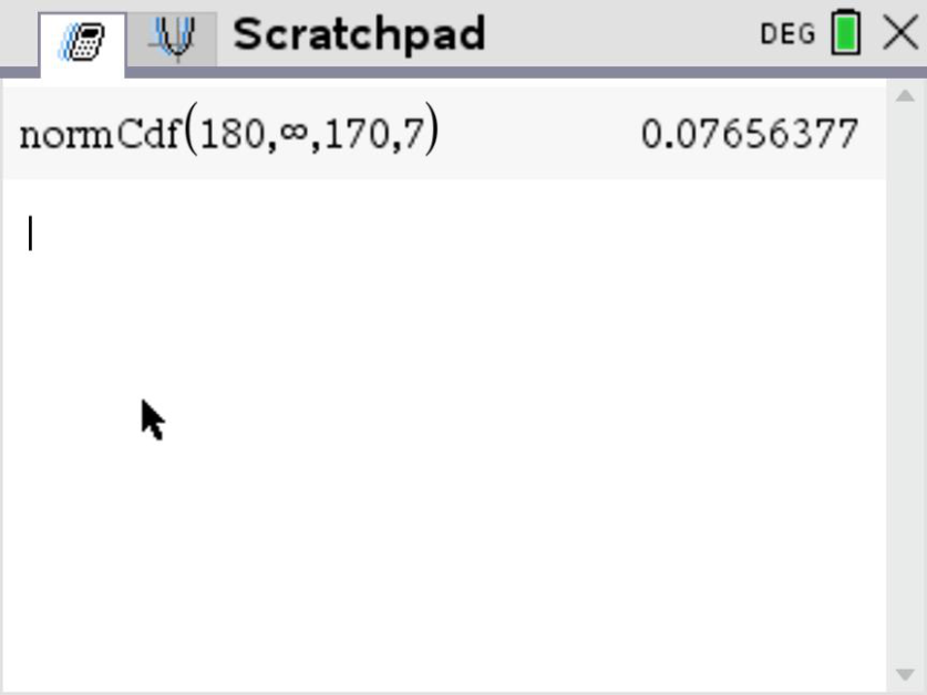
\[\mathrm{P}(X>180)=\operatorname{normCdf}(180,\infty,170,7)\approx\boxed{0.0766}.\] The display gives \(0.07656377\), so approximately \(7.66\%\) of the population measures more than \(180\) cm.
All four probabilities match the histogram areas in Appendix A: the calculator now finds the area for us.
Apply the method to other normal models
Normal models also describe other measurements. We now consider the operating time of a battery under fixed test conditions. The method stays the same: read the model, choose the bounds and calculate the area.
Worked example 6 — three types of probability
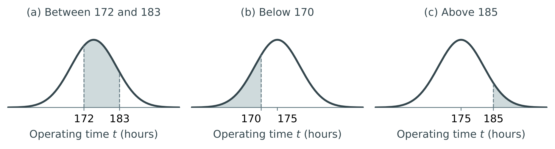
Question. The operating time \(T\), in hours, of a battery under fixed test conditions is modelled by \(T\sim\mathrm{N}(175,7^2)\). Find:
(a) \(\mathrm{P}(172<T<183)\);
(b) \(\mathrm{P}(T<170)\);
(c) \(\mathrm{P}(T>185)\).
Solution
(a) \(\mathrm{P}(172<T<183)=\operatorname{normCdf}(172,183,175,7)\approx\boxed{0.539}\).
(b) The left tail starts at \(-\infty\): \[\mathrm{P}(T<170)=\operatorname{normCdf}(-\infty,170,175,7) =0.237525\ldots\approx\boxed{0.238}.\]
(c) The right tail ends at \(+\infty\): \[\mathrm{P}(T>185)=\operatorname{normCdf}(185,\infty,175,7) =0.0765637\ldots\approx\boxed{0.0766}.\]
Enter the standard deviation, not the variance
For \(T\sim\mathrm{N}(175,49)\), enter \(\sigma=7\), not \(49\). Use the infinity symbol in a tail bound, or a sufficiently large substitute such as \(-10^9\) or \(10^9\) for the scales used here.
Probability, percentage and expected number
A probability \(p\) corresponds to a percentage \(100p\%\). In a group of \(n\) observations, the expected number satisfying the condition is \(np\).
Worked example 7 — rejected cartons
Question. Milk volume \(V\), in ml, follows \(V\sim\mathrm{N}(500,6^2)\). A carton is rejected if it contains less than \(492\) ml.
(a) Find the rejection probability.
(b) Estimate the number rejected out of \(240\) cartons.
Solution
(a) \(p=\mathrm{P}(V<492)=\operatorname{normCdf}(-\infty,492,500,6)=0.0912112\ldots\approx\boxed{0.0912}\).
(b) Expected number \(=np=240(0.0912112\ldots)=21.8907\ldots\). We expect approximately 22 cartons to be rejected. This is an estimate, not a guarantee. Use the unrounded probability in the multiplication.
Inverse normal: start with an area, find a value
A normal CDF calculation starts with boundaries and finds a probability. An inverse normal calculation starts with a probability and finds a boundary.
The left tail rule

If \(X\sim\mathrm{N}(\mu,\sigma^2)\) and \(\mathrm{P}(X<k)=p\), then \[k=\operatorname{invNorm}(p,\mu,\sigma),\qquad 0<p<1.\] Always enter the left-tail area \(p\). If the right-tail area is \(q\), use \(p=1-q\).
TI-Nspire CX: in the calculation Scratchpad, choose Menu \(\longrightarrow\) Probability \(\longrightarrow\) Distributions \(\longrightarrow\) Inverse Normal. Enter Area, \(\mu\) and \(\sigma\).
Worked example 8 — percentiles and the tallest 10%
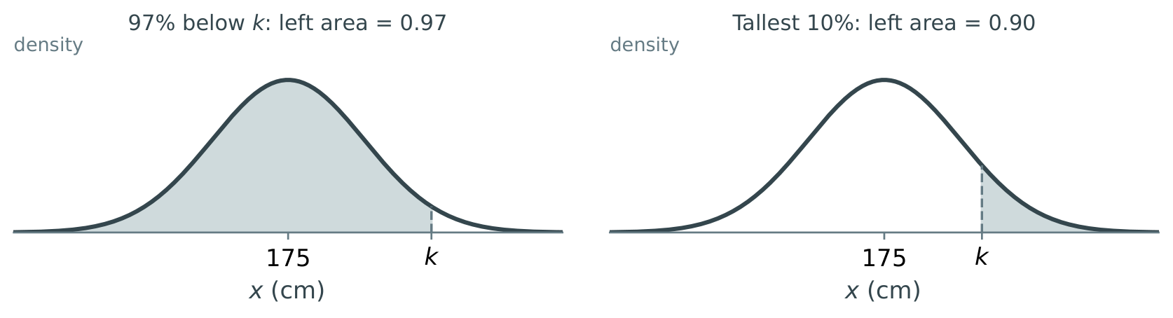
Question. In a height model, \(X\sim\mathrm{N}(175,7^2)\), with \(X\) in cm.
(a) Find the height below which \(97\%\) of the population lies.
(b) Find the threshold for the tallest \(10\%\) of the population.
Solution
(a) Write the probability statement: \(\mathrm{P}(X<k)=0.97\). Then \[k=\operatorname{invNorm}(0.97,175,7)=188.1656\ldots\text{ cm}.\] The \(97\)th percentile is approximately 188 cm (3 s.f.). This means about \(97\%\) lie below that height, not that the height itself is a probability.
(b) We have \(\mathrm{P}(X>k)=0.10\), so \(\mathrm{P}(X<k)=0.90\). Thus \[k=\operatorname{invNorm}(0.90,175,7)=183.9709\ldots\text{ cm}.\] The cut-off is approximately 184 cm (3 s.f.). The unrounded model threshold is \(183.9709\ldots\) cm; rounding does not change the exact condition being modelled.
A quick sense check
A percentile above \(50\%\) must lie above the mean. Both \(97\%\) and \(90\%\) are greater than \(50\%\), so both answers must exceed \(175\) cm.
Inverse normal when the area is not a left tail
Worked example 9 — an area starting at the mean
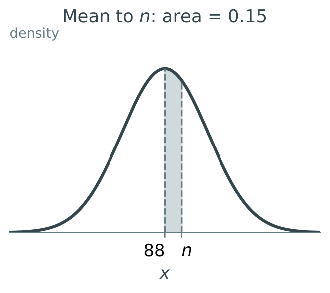
Question. \(X\sim\mathrm{N}(88,19^2)\). Find \(n\) such that \(\mathrm{P}(88<X<n)=0.15\).
Solution
The mean is \(88\), so \(\mathrm{P}(X<88)=0.50\). Add the shaded strip to this left half: \[\mathrm{P}(X<n)=0.50+0.15=0.65.\] Now use the whole left area: \[\begin{aligned} n&=\operatorname{invNorm}(0.65,88,19)\\ &=95.3211\ldots\approx\boxed{95.3}. \end{aligned}\] The answer is above \(88\), as the diagram requires.
Worked example 10 — the central 95%
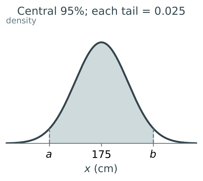
Question. \(X\sim\mathrm{N}(175,7^2)\). Find the interval symmetric about the mean containing exactly \(95\%\) of the model’s probability.
Solution
The total area outside the interval is \(1-0.95=0.05\). Symmetry gives two equal tails, each with area \(0.025\).
Do not put 0.95 into both inverse calculations
The inverse command requires cumulative left areas: \(0.025\) at the lower end and \(0.975\) at the upper end. The rough 68–95–99.7 rule gives \(175\pm14\); the calculator interval is slightly narrower.
The same idea for any central proportion
For a central proportion \(c\), the two tail areas are \((1-c)/2\). The left areas to enter are \((1-c)/2\) and \((1+c)/2\).
For example: the central \(80\%\) leaves \(10\%\) in each tail, so use \(0.10\) and \(0.90\).
Why specify “central”? An area of \(0.95\) alone does not determine both endpoints of an interval. Symmetry about the mean supplies the second condition.
Connect the ideas and interpret the model
We now combine normal probabilities with conditional probability: the condition changes the group from which we select.
Worked example 11 — “given that” changes the group
Consolidation with conditional probability (SL 4.11).
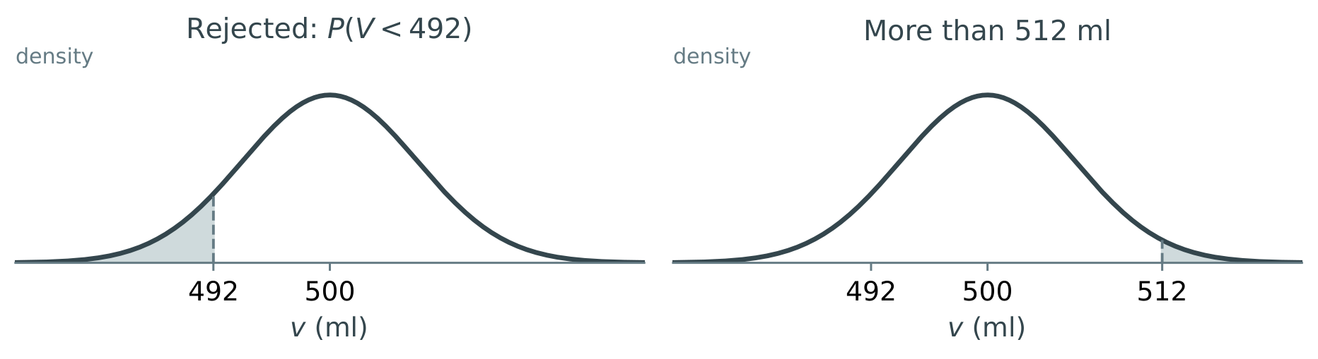
Milk volume \(V\sim\mathrm{N}(500,6^2)\) ml. A carton is rejected if \(V<492\).
Question. Given that a carton is not rejected, find the probability that it contains more than \(512\) ml.
Solution
We now choose from the accepted cartons only. Let \(A\) mean \(V>512\) and \(B\) mean \(V\geq492\). Every carton in \(A\) is also in \(B\), so \(A\cap B=A\).
\[\begin{aligned} \mathrm{P}(A\mid B)&=\frac{\mathrm{P}(A\cap B)}{\mathrm{P}(B)}\\[2pt] &=\frac{\mathrm{P}(V>512)}{\mathrm{P}(V\geq492)}\\[2pt] &=\frac{0.0227501\ldots}{1-0.0912112\ldots}\\[2pt] &=0.0250335\ldots\approx\boxed{0.0250}. \end{aligned}\] About 2.50% of accepted cartons contain more than \(512\) ml. The denominator is the probability of the condition after “given that”.What does a normal model assume?
The population is approximately symmetric and bell-shaped, with the stated mean and standard deviation. Check the context or data before choosing this model.
A normal curve permits every real value. For a physical quantity such as height or volume, the model is useful when the probability of impossible values is negligible.
A probability describes a long-run proportion. A finite sample need not match it exactly.
Common mistakes to catch
Do not use the curve’s height as a probability. Do not enter the
variance in the standard-deviation field. Do not use a right-tail area
directly in invNorm. Keep unrounded calculator values until
the final answer.
Practice
Use a calculator except where the 68–95–99.7 rule is requested. Give numerical probabilities and values to 3 significant figures, unless instructed otherwise. Sketch and shade each probability or inverse-normal event. Work on separate paper.
\(X\sim\mathrm{N}(60,25)\).
(a) State \(\mu\) and \(\sigma\).
(b) Explain what happens to the curve if \(\sigma\) increases to \(8\) while \(\mu\) stays unchanged.
Check answer 1\(X\sim\mathrm{N}(100,15^2)\). Use the 68–95–99.7 rule to estimate:
(a) \(\mathrm{P}(85<X<115)\);
(b) \(\mathrm{P}(X>130)\);
(c) \(\mathrm{P}(70<X<115)\).
Check answer 2(a) Explain why \(\mathrm{P}(X=100)=0\) for a normal variable.
(b) Does \(\mathrm{P}(X<100)\) differ from \(\mathrm{P}(X\leq100)\)? Explain.
Check answer 3\(X\sim\mathrm{N}(50,8^2)\). Find:
(a) \(\mathrm{P}(X<58)\);
(b) \(\mathrm{P}(X>45)\);
(c) \(\mathrm{P}(42<X<60)\).
Check answer 4The mass \(M\) of a packet, in grams, follows \(M\sim\mathrm{N}(200,4^2)\).
(a) Find \(\mathrm{P}(M<194)\).
(b) Estimate the number below \(194\) g among \(600\) packets.
(c) Explain why your estimate need not equal the actual number.
Check answer 5\(X\sim\mathrm{N}(60,5^2)\). Find:
(a) \(k\) such that \(\mathrm{P}(X<k)=0.35\);
(b) \(m\) such that \(\mathrm{P}(X>m)=0.15\);
(c) \(n\) such that \(\mathrm{P}(60<X<n)=0.20\).
Check answer 6\(X\sim\mathrm{N}(100,15^2)\). Find the central \(80\%\) interval. State both endpoints to 1 decimal place.
Check answer 7\(X\sim\mathrm{N}(100,15^2)\). A student’s solution says \(\mathrm{P}(X>k)=0.08\), therefore \(k=\operatorname{invNorm}(0.08,100,15)\).
(a) Explain the error.
(b) Find the correct value of \(k\).
Check answer 8Milk volume \(V\sim\mathrm{N}(500,6^2)\) ml. Cartons with \(V<492\) are rejected. Given that a carton is accepted, find the probability that its volume exceeds \(510\) ml.
Consolidation with conditional probability.
Check answer 9A delivery company proposes a normal model for waiting times. The data have many short waits and a few extremely long waits.
(a) Explain why a normal model may be unsuitable.
(b) If \(T\sim\mathrm{N}(3,4^2)\) minutes were used, calculate \(\mathrm{P}(T<0)\) and explain what this suggests about the model.
Check answer 10
Answers and working
(a) \(\mu=60\), \(\sigma=\sqrt{25}=5\).
(b) The curve becomes wider and lower; its centre stays at \(60\) and its total area stays \(1\).
(a) The interval is \(\mu\pm\sigma\), so \(\mathrm{P}(85<X<115)\approx0.68\).
(b) \(130=\mu+2\sigma\), so \(\mathrm{P}(X>130)\approx(1-0.95)/2=0.025\).
(c) Split at \(100\): \(0.95/2+0.68/2=0.475+0.34=0.815\).
(a) A single point has zero width and hence zero area beneath a continuous density curve.
(b) No: including the single point adds a probability of zero.
(a) \(\operatorname{normCdf}(-\infty,58,50,8)=0.8413447\ldots\approx\boxed{0.841}\).
(b) \(\operatorname{normCdf}(45,\infty,50,8)=0.7340145\ldots\approx\boxed{0.734}\).
(c) \(\operatorname{normCdf}(42,60,50,8)=0.7356950\ldots\approx\boxed{0.736}\).
(a) \(p=\operatorname{normCdf}(-\infty,194,200,4)=0.0668072\ldots\approx\boxed{0.0668}\).
(b) Expected number \(=600p=40.0843\ldots\), so approximately 40 packets.
(c) Random variation means the observed count may differ from its expected value.
(a) \(k=\operatorname{invNorm}(0.35,60,5)=58.0734\ldots\approx\boxed{58.1}\).
(b) Left area \(=1-0.15=0.85\). Thus \(m=\operatorname{invNorm}(0.85,60,5)=65.1822\ldots\approx\boxed{65.2}\).
(c) Left area \(=0.50+0.20=0.70\). Thus \(n=\operatorname{invNorm}(0.70,60,5)=62.6220\ldots\approx\boxed{62.6}\).
Each tail has area \((1-0.80)/2=0.10\). The endpoints are \[\operatorname{invNorm}(0.10,100,15)=80.7767\ldots,\qquad \operatorname{invNorm}(0.90,100,15)=119.2233\ldots.\] The central interval is \([80.8,119.2]\) to 1 decimal place.
(a) \(0.08\) is a right-tail area;
invNormrequires the left area, \(0.92\).(b) \(k=\operatorname{invNorm}(0.92,100,15)=121.0761\ldots\approx\boxed{121}\). Since only \(8\%\) lie above \(k\), it must be above the mean.
We restrict to accepted cartons, \(V\geq492\): \[\mathrm{P}(V>510\mid V\geq492) =\frac{\mathrm{P}(V>510)}{\mathrm{P}(V\geq492)} =\frac{0.0477904\ldots}{0.9087888\ldots} \approx\boxed{0.0526}.\]
(a) The described data are skewed to the right, whereas a normal distribution is symmetric.
(b) \(\mathrm{P}(T<0)=\operatorname{normCdf}(-\infty,0,3,4)=0.226627\ldots\approx\boxed{0.227}\). The model assigns about \(22.7\%\) probability to impossible negative waits, a serious reason to reject it.
Quick reference and tutorial library
| Task | Set-up | Calculator method |
|---|---|---|
| Probability below \(k\) | \(\mathrm{P}(X<k)\) | \(\operatorname{normCdf}(-\infty,k,\mu,\sigma)\) |
| Probability above \(k\) | \(\mathrm{P}(X>k)\) | \(\operatorname{normCdf}(k,\infty,\mu,\sigma)\) |
| Probability between | \(\mathrm{P}(a<X<b)\) | \(\operatorname{normCdf}(a,b,\mu,\sigma)\) |
| Cut-off: left area \(p\) | \(\mathrm{P}(X<k)=p\) | \(\operatorname{invNorm}(p,\mu,\sigma)\) |
| Cut-off: right area \(q\) | \(\mathrm{P}(X>k)=q\) | \(\operatorname{invNorm}(1-q,\mu,\sigma)\) |
| Expected number | \(n\) observations; probability \(p\) | \(np\) |
Before you calculate: define the variable, identify \(\mu\) and \(\sigma\), sketch, label and shade.
After you calculate: check the size of the area or the position of the boundary; give units where appropriate; round only at the end.
What belongs to the next handout?
Standardising with \(z=(x-\mu)/\sigma\) and finding unknown means or standard deviations belong to AA SL 4.12, studied by both AA SL and AA HL. They are developed in the companion handout.
Adapted from John Radford’s normal-distribution, empirical-rule and inverse-normal webpage exports and the linked Radford Mathematics tutorials. Syllabus scope checked against the supplied IB guide, SL 4.9. Calculator command names follow the TI-Nspire distribution reference.
From wide rectangles to a smooth bell curve
Optional exploration. Follow the same shaded interval through narrower histograms, then compare histogram and bell-curve probabilities using a full table.
Let \(X\) be the height, in cm, of a randomly selected person. Height is a continuous random variable: it is a measurement that can take any value within an interval.
Bell-shaped patterns occur in many contexts. Heights within a comparable group, weights of manufactured products and some test scores can be approximately normally distributed: values cluster around a centre, with fewer far below or above it. We check the data before choosing this model.
For the same ideal normal population as in section 1, the histogram bars and the curve represent one model of heights. We want to know: what percentage of people have heights between \(160\) and \(180\) cm?
In each histogram below, a rectangle’s area equals the percentage of the population in its class interval. Add the shaded rectangle areas to find the percentage between \(160\) and \(180\). All the rectangle areas together represent \(100\%\).
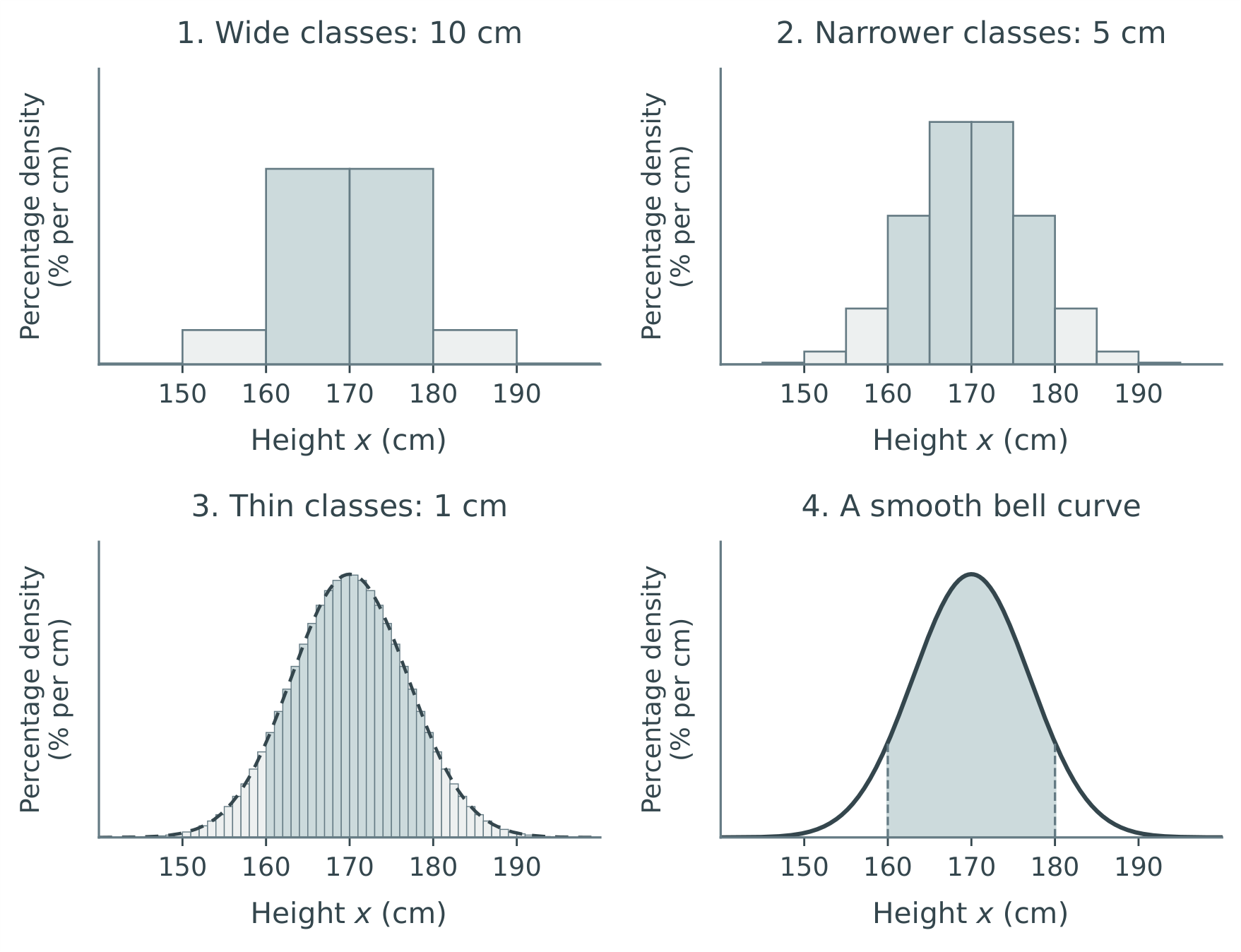
Follow the same shaded interval through all four graphs. Narrower classes give thinner rectangles. In this ideal model, as their widths tend to zero, their tops trace a smooth bell curve. With total area \(1=100\%\), the curve is the graph of a probability density function (pdf).
Keep the histogram picture in mind. The percentage between \(160\) and \(180\) is still represented by an area. The bell curve replaces the outline of the increasingly thin rectangles, and finding the area under it replaces adding their areas. The question and the shaded interval stay the same.
Read probabilities from the full histogram table
We can calculate probabilities from the histogram and compare each result with the corresponding bell-curve area.
The total area of all the rectangles, or under the bell curve, is \(1=100\%\). The area of one rectangle, or the sum of several rectangle areas, is the probability of the corresponding interval.
The table matches the 1 cm classes in graph 3 in Appendix A.1. It lists population percentages to four decimal places, with the extreme tails grouped into two entries.
| Height class (cm) | Population (%) | Height class (cm) | Population (%) |
|---|---|---|---|
| \(150\leq x<151\) | \(0.1184\) | \(170\leq x<171\) | \(5.6798\) |
| \(151\leq x<152\) | \(0.1743\) | \(171\leq x<172\) | \(5.5653\) |
| \(152\leq x<153\) | \(0.2515\) | \(172\leq x<173\) | \(5.3431\) |
| \(153\leq x<154\) | \(0.3556\) | \(173\leq x<174\) | \(5.0263\) |
| \(154\leq x<155\) | \(0.4927\) | \(174\leq x<175\) | \(4.6329\) |
| \(155\leq x<156\) | \(0.6688\) | \(175\leq x<176\) | \(4.1842\) |
| \(156\leq x<157\) | \(0.8895\) | \(176\leq x<177\) | \(3.7028\) |
| \(157\leq x<158\) | \(1.1593\) | \(177\leq x<178\) | \(3.2106\) |
| \(158\leq x<159\) | \(1.4803\) | \(178\leq x<179\) | \(2.7278\) |
| \(159\leq x<160\) | \(1.8522\) | \(179\leq x<180\) | \(2.2708\) |
| \(160\leq x<161\) | \(2.2708\) | \(180\leq x<181\) | \(1.8522\) |
| \(161\leq x<162\) | \(2.7278\) | \(181\leq x<182\) | \(1.4803\) |
| \(162\leq x<163\) | \(3.2106\) | \(182\leq x<183\) | \(1.1593\) |
| \(163\leq x<164\) | \(3.7028\) | \(183\leq x<184\) | \(0.8895\) |
| \(164\leq x<165\) | \(4.1842\) | \(184\leq x<185\) | \(0.6688\) |
| \(165\leq x<166\) | \(4.6329\) | \(185\leq x<186\) | \(0.4927\) |
| \(166\leq x<167\) | \(5.0263\) | \(186\leq x<187\) | \(0.3556\) |
| \(167\leq x<168\) | \(5.3431\) | \(187\leq x<188\) | \(0.2515\) |
| \(168\leq x<169\) | \(5.5653\) | \(188\leq x<189\) | \(0.1743\) |
| \(169\leq x<170\) | \(5.6798\) | \(189\leq x<190\) | \(0.1184\) |
| \(x<150\) | \(0.2137\) | \(x\geq190\) | \(0.2137\) |
Rounding affects the total; exact endpoints add no area and do not change probabilities.
Appendix example A1 — one bar, an interval and two tails
Question. Use the table to find:
(a) \(\mathrm{P}(170<X<171)\);
(b) \(\mathrm{P}(160<X<180)\);
(c) \(\mathrm{P}(X<165)\);
(d) \(\mathrm{P}(X>180)\).
Reading the notation: \(\mathrm{P}(170<X<171)\) means “the probability that the randomly selected person measures between \(170\) and \(171\) cm.”
Solution
(a) One bar. The class from \(170\) to \(171\) cm contains \(5.6798\%\) of the population: \[\mathrm{P}(170<X<171)\approx5.6798\%=0.056798\approx\boxed{0.0568}.\] The shaded areas in the two graphs represent the same probability.

Solutions (b)–(d). Add the relevant percentages and state the decimal equivalent. Compare each shaded histogram region with the bell-curve region beside it.
(b) Between two values. Add the percentages for the \(20\) bars from \(160\) to \(180\): \[\begin{aligned} (2.2708+2.7278+\cdots+2.7278+2.2708)\%&=84.6872\%=0.846872,\\ \mathrm{P}(160<X<180)&\approx\boxed{0.847}. \end{aligned}\]

(c) A left tail. Add the lower tail percentage and the percentages for every bar below \(165\): \[\begin{aligned} (0.2137+0.1184+\cdots+4.1842)\%&=23.7525\%=0.237525,\\ \mathrm{P}(X<165)&\approx\boxed{0.238}. \end{aligned}\]

(d) A right tail. Add the percentages for every bar above \(180\) and the upper tail: \[\begin{aligned} (1.8522+1.4803+\cdots+0.1184+0.2137)\%&=7.6563\%=0.076563,\\ \mathrm{P}(X>180)&\approx\boxed{0.0766}. \end{aligned}\]

These histogram calculations give the same probabilities as the normal model in the main lesson. The same questions can be phrased as follows.
The same example — how it might appear in a test
The heights of people in a population are normally distributed with a mean of \(170\) cm and a standard deviation of \(7\) cm. A person is selected at random. Find the probability that this person’s height is:
(a) between \(170\) cm and \(171\) cm;
(b) between \(160\) cm and \(180\) cm;
(c) less than \(165\) cm;
(d) greater than \(180\) cm.
The questions and shaded areas are unchanged. What distinguishes one normal distribution from another is its mean \(\mu\) and standard deviation \(\sigma\). These two parameters determine its equation, as shown in section 2.