IB Mathematics: Applications and Interpretation SL · Topic 4
Presentation of Data
From a table of observations to a clear graph, a meaningful summary and a justified comparison.
Learning goal
Organize data, construct and read statistical diagrams, and justify comparisons in context.
Syllabus link
AI SL: SL 4.2. Frequency tables, histograms, cumulative frequency, quartiles, percentiles and box plots.
Big idea
Each representation answers a different question about the same data. Choose the graph for the information you need.
Technology and interpretation
Use a graphical calculator for statistical summaries. A GDC is required for both AI SL papers; show your method and interpret the output.
A complete online lesson with explanations, worked examples, original IB-style walkthroughs, practice and full answers. Use a notebook and squared paper for the drawing tasks. Calculator screenshots use the TI-Nspire CX.
One data set, several useful pictures. A long raw list hides patterns. A frequency table organizes the counts; these three displays make particular features easier to see.
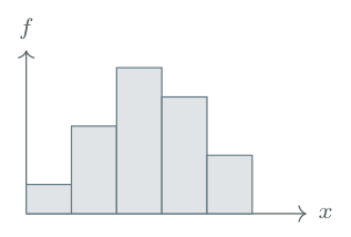
Histogram
Which intervals are common? What is the overall shape?
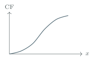
Cumulative frequency
How many lie below a value? Where are the percentiles?
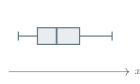
Box plot
How do centre and spread compare? Are there unusual values?
How to use this lesson
Study each explanation and worked example, then attempt the checkpoint. Use a calculator for numerical summaries and a notebook or squared paper for working and graphs. Attempt the new-data practice independently before checking the answers. Videos are optional support.
Scope. Aligned with AI SL 4.2 in the guide first assessed in 2021. Frequency-density histograms are not required; their tutorial is optional enrichment. The raw-data quartile recap supports this section and links to 4.3. All IB-style questions are original; marks are suggested, not an official IB markscheme.
Data and frequency distributions
Begin with the variable
A variable is the quantity recorded for each observation. Discrete numerical data have separate, countable possible values, such as numbers of books. Continuous data can take any value in an interval, such as time or height; recorded values may be rounded.
A frequency is the number of times a value, or a class of values, occurs. A frequency table keeps the counts without listing every repeated observation. The total frequency is the number of observations, \(n\). \[\sum f=n.\qquad \text{Percentage in a group}=\frac{\text{frequency in that group}}{n}\times100\%.\]
Worked example 1: organize a raw list
The numbers of books read by 20 students in a month are 1, 2, 2, 3, 4, 2, 1, 0, 3, 2, 4, 3, 1, 2, 5, 3, 2, 4, 1, 3.
Construct a frequency table.
State the modal number of books.
Find the percentage who read at least three books.
Step-by-step solution
Solution
(a) Frequency table
Count each observation once. Include zero as a possible observed value.
| Books, \(x\) | 0 | 1 | 2 | 3 | 4 | 5 | Total |
|---|---|---|---|---|---|---|---|
| Frequency, \(f\) | 1 | 4 | 6 | 5 | 3 | 1 | 20 |
Check: \(1+4+6+5+3+1=20\), so all observations are accounted for.
(b) Mode
The mode is the value with the largest frequency. The largest frequency is 6, so the mode is 2 books, not 6 books.
(c) Percentage
“At least three” includes 3, 4 and 5. Their total frequency is \(5+3+1=9\). \[\frac{9}{20}\times100\%=45\%.\]
Values and counts are different
In the table, \(x=2\) is a number of books; \(f=6\) is a number of students. The mean, median and mode of a variable are data values, not frequencies. More than one value can be a mode if the largest frequency is shared.
Median, quartiles and spread: the foundations
What the summary values mean
The median is the centre of the ordered data. The lower quartile, \(Q_1\), marks the lower quarter, and the upper quartile, \(Q_3\), marks the upper quarter. The median is also \(Q_2\). \[\text{Range}=\text{maximum}-\text{minimum},\qquad \operatorname{IQR}=Q_3-Q_1.\] The range describes the full spread. The IQR describes the spread of the middle half and is less sensitive to extreme observations.
Raw data: order first, then locate the middle
Put the observations in ascending order, keeping repeated values. Number their positions \(1,2,\ldots,n\). The middle of the list is at \[\boxed{\text{middle position}=\frac{n+1}{2}}.\] Odd \(n\): the position is a whole number, so take the value in that position.
Even \(n\): the position is halfway between two whole numbers, so average the values in those two positions.
For the median-of-halves method used here, \(Q_1\) is the median of the lower half and \(Q_3\) is the median of the upper half. When \(n\) is odd, exclude the overall median from both halves.
These hand calculations explain the ideas. In AI SL, use technology for numerical summaries. Quartile conventions can differ: follow the question and use one method consistently.
Foundation example A: eight values — even \(n\)
The ordered scores are \(2,4,5,7,8,10,12,16\).
Find the median, \(Q_1\) and \(Q_3\).
Find the range and IQR.
Step-by-step solution
Solution
(a) Locate the middle, then find the median and quartiles
There are \(n=8\) observations, so \[\text{middle position}=\frac{n+1}{2}=\frac{8+1}{2}=4.5.\] Position \(4.5\) lies between the 4th and 5th observations, whose values are 7 and 8. Average these values, not their position numbers.
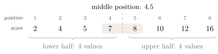
Each half has 4 values. Its middle position is \((4+1)/2=2.5\), so average the second and third values of that half to find its median. \[\begin{aligned} \text{Median}&=\frac{7+8}{2}=7.5,\\ Q_1&=\frac{4+5}{2}=4.5,\\ Q_3&=\frac{10+12}{2}=11. \end{aligned}\]
(b) Range and interquartile range
Range \(=16-2=\boxed{14}\); IQR \(=11-4.5=\boxed{6.5}\).
Foundation example B: nine values — odd \(n\)
The ordered scores are \(2,4,5,7,8,10,12,14,16\).
Find the median, \(Q_1\) and \(Q_3\).
Find the range and IQR.
Step-by-step solution
Solution
(a) Locate the middle, then find the median and quartiles
There are \(n=9\) observations, so \[\text{middle position}=\frac{n+1}{2}=\frac{9+1}{2}=5.\] The 5th observation is 8, so the median is 8. The number 5 tells us where to look; it is not the median score.
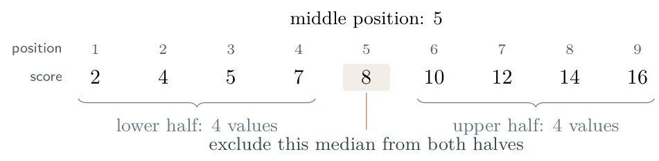
Using our median-of-halves convention, leave out the overall median, 8, when forming the two halves: \[\text{lower half: }2,4,5,7,\qquad \text{upper half: }10,12,14,16.\] Each half has 4 values. Its middle position is \((4+1)/2=2.5\), so average the second and third values within that half. \[\begin{aligned} \text{Median}&=8,\\ Q_1&=\frac{4+5}{2}=4.5,\\ Q_3&=\frac{12+14}{2}=13. \end{aligned}\]
(b) Range and interquartile range
Range \(=16-2=\boxed{14}\); IQR \(=13-4.5=\boxed{8.5}\).
One position formula, two ways to read the list
For \(n=8\), position \(4.5\) means average the 4th and 5th values. For \(n=9\), position \(5\) means take the 5th value. In both cases, \((n+1)/2\) gives a position, not the median itself.
Raw-list positions are not cumulative-frequency levels
Use \((n+1)/2\) to locate the middle of a raw ordered list. For grouped cumulative-frequency graphs, use levels \(n/4\), \(n/2\) and \(3n/4\) on the vertical axis, then read data values on the horizontal axis. Do not substitute \((n+1)/2\) for the graph’s median level \(n/2\).
IB-style walkthrough A: values with frequencies
[10 marks]
The following table shows the number of books borrowed by each of 30 students during one month.
| Books borrowed, \(x\) | 0 | 1 | 2 | 3 | 4 |
|---|---|---|---|---|---|
| Frequency, \(f\) | 3 | 7 | 11 | 6 | 3 |
State whether the variable is discrete or continuous. Give a reason.[2]
Write down the mode.[1]
Determine the median.[2]
Use technology to find \(Q_1\) and \(Q_3\). Hence find the IQR.[3]
Calculate the percentage of students who borrowed at least three books.[2]
Step-by-step solution
Solution
(a) Type of data
The variable is discrete: books are counted and the possible values are separate whole numbers.
(b) Mode
The greatest frequency is 11, attached to \(x=2\). The mode is 2 books.
(c) Median
Enter \(0,1,2,3,4\) as the data list and \(3,7,11,6,3\) as its frequency list. One-Variable Statistics gives \(n=30\) and median \(2\). To understand this output, locate the positions in the ordered list:
| Books | 0 | 1 | 2 | 3 | 4 |
|---|---|---|---|---|---|
| Positions in ordered list | 1–3 | 4–10 | 11–21 | 22–27 | 28–30 |
The central observations are the 15th and 16th. Both are 2, so \[\text{median}=\frac{2+2}{2}=2\text{ books}.\]
(d) Quartiles and IQR
The same calculator output gives \(Q_1=1\) and \(Q_3=3\). As a check, the lower and upper halves each have 15 observations: their medians are the 8th and 23rd observations overall, with values 1 and 3. \[\operatorname{IQR}=3-1=2\text{ books}.\]
(e) Percentage
There are \(6+3=9\) students with at least three books, so \[\frac{9}{30}\times100\%=30\%.\]
What earns the method marks?
State the relevant statistics and show any subsequent calculation or interpretation. Use the frequency list, not just the five column labels. A correct calculator output does not replace the explanation requested in the question.
Calculator procedure. The illustrated data-list and frequency-list workflow is in 7.2: frequency-table calculator guide–7.2: frequency-weighted box plot. The calculations by hand above explain the output.
Grouped data and equal-width histograms
Continuous data are often grouped into class intervals. Class boundaries tell us where each interval starts and ends; its width is upper boundary minus lower boundary.

A filled endpoint is included; an open endpoint is excluded. Thus \(t=20\) belongs to \(20\le t<30\), not to \(10\le t<20\). Some questions use \(a<t\le b\) instead: always follow the stated inequalities.
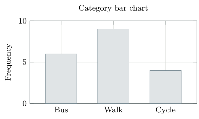
A histogram is not a category bar chart
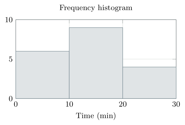
A histogram uses a continuous numerical scale and shows the frequency in each class. Adjacent non-zero bars meet at their class boundary. With equal class widths, the vertical axis can be frequency and each bar’s height is the class frequency.
Constructing a histogram
Check that the classes cover the data without gaps or overlaps, and have equal widths.
Mark the class boundaries on a numerical horizontal scale; label the variable and units.
Label the vertical axis Frequency. Choose a scale reaching the largest frequency.
Draw each rectangle across its whole interval, with height equal to its frequency.
The modal class is the interval with the greatest frequency. Grouping does not reveal the exact mode or the exact individual observations.
A genuine empty class is different from decorative gaps
A class with frequency zero has no visible bar. Leave its full interval on the scale. Do not insert arbitrary gaps between non-zero bars as you would in a category chart. Frequency-density methods for unequal widths are outside the required AI SL 4.2 content.
Constructing and interpreting a histogram
Worked example 2: travel times to school
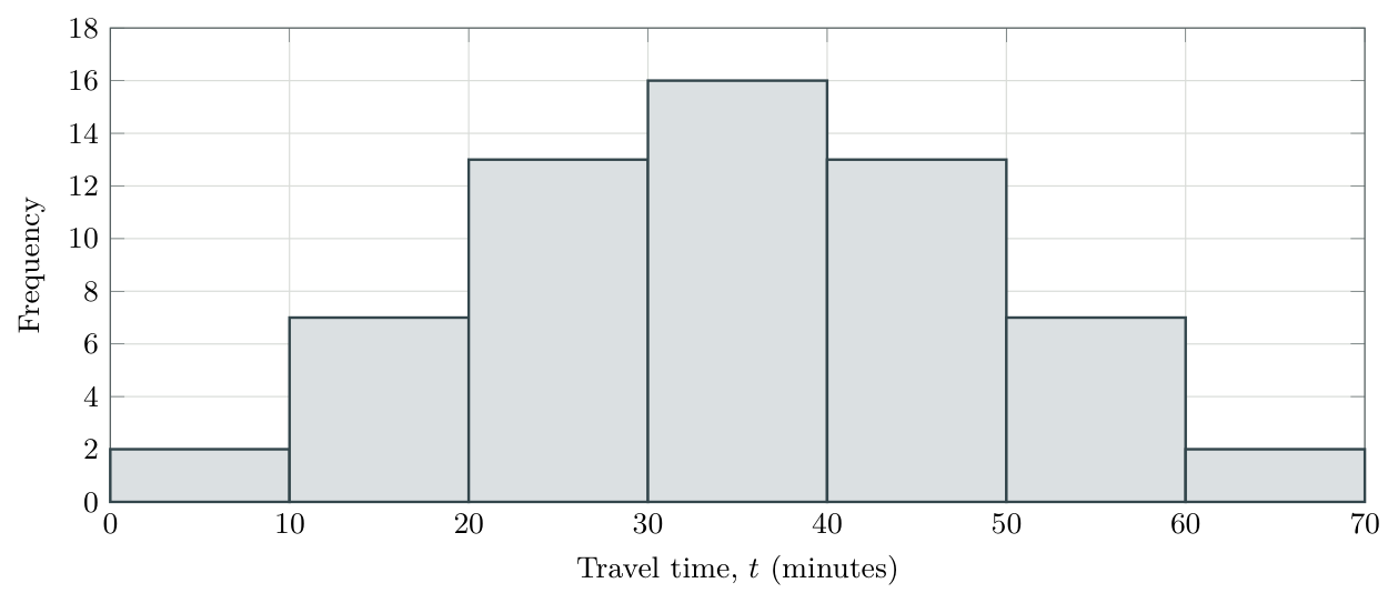
The travel times to school for 60 students are summarized below.
| \(t\) (min) | \(0\le t<10\) | \(10\le t<20\) | \(20\le t<30\) | \(30\le t<40\) | \(40\le t<50\) | \(50\le t<60\) | \(60\le t<70\) |
|---|---|---|---|---|---|---|---|
| Frequency | 2 | 7 | 13 | 16 | 13 | 7 | 2 |
Draw a frequency histogram.
State the modal class.
Find the number whose travel time is at least 20 minutes but less than 50 minutes.
Describe the overall shape. Can the exact median be recovered from this table?
Step-by-step solution
Solution
(a) Histogram
Each interval has width 10 minutes. Mark \(0,10,\ldots,70\) at the edges of the bars; use the frequencies as heights.
(b) Modal class
The greatest frequency is 16, so the modal class is \(\boxed{30\le t<40}\) minutes.
(c) Number of students
The interval \(20\le t<50\) includes three complete classes. Add their frequencies: \[13+16+13=\boxed{42\text{ students}}.\]
(d) Shape and limitations
The histogram is symmetric about 35 minutes and has one central peak. The grouped table does not give the exact median: we do not know the positions of the observations inside their intervals. A cumulative-frequency graph will let us estimate it.
Read the request before calculating
Counts for whole classes come directly from the table and are exact. A threshold inside a class usually requires an estimate. A class interval is not a list of observations all equal to its midpoint.
IB-style walkthrough B: a histogram question
[8 marks]
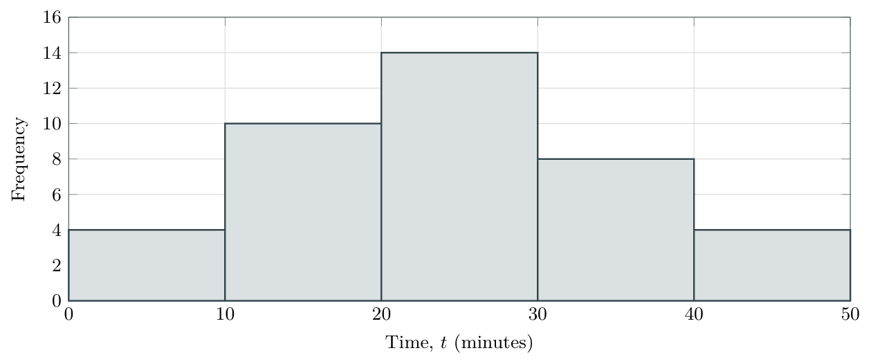
A researcher records the time \(t\), in minutes, taken by 40 students to complete a task.
| \(t\) (minutes) | \(0\le t<10\) | \(10\le t<20\) | \(20\le t<30\) | \(30\le t<40\) | \(40\le t<50\) |
|---|---|---|---|---|---|
| Frequency | 4 | 10 | 14 | 8 | 4 |
Draw a frequency histogram.[3]
State the modal class.[1]
Determine the percentage who took at least 30 minutes.[2]
Describe the overall shape, giving a reason.[2]
Step-by-step solution
Solution
(a) Construct the diagram
The rectangles have width 10 minutes and heights \(4,10,14,8,4\). The scale is labelled at every class boundary, including the final boundary 50.
(b) Modal class
The tallest bar spans \(20\le t<30\), so this is the modal class.
(c) Percentage
“At least 30” includes both final classes. There are \(8+4=12\) students: \[\frac{12}{40}\times100\%=\boxed{30\%}.\]
(d) Shape
The distribution is approximately symmetric with one peak: frequencies rise towards the central class and fall on either side. The outer pair is equal; the next pair, 10 and 8, is similar but not identical.
What the diagram does not establish
Do not claim the exact mode is 25 minutes, or that this is certainly a normal distribution. The data identify an interval with the greatest frequency and suggest a shape, not the exact values within that interval.
Cumulative frequency: building the graph
Plot the upper boundary, not the midpoint
Cumulative frequency is a running total. With intervals written \(a\le x<b\), it counts observations below the upper boundary \(b\). Each class contributes the point \[\boxed{(\text{class upper boundary},\ \text{cumulative frequency})}.\] Also plot the starting point \((\text{first lower boundary},0)\). This is an extra starting point, not a class upper-boundary point.
Construction and checks
Add the frequencies cumulatively; plot upper boundaries horizontally and running totals vertically. Start at cumulative frequency zero and finish at \(n\). The graph must never decrease; a zero-frequency class produces a horizontal segment.
For the hand-drawn diagrams in this lesson, join the plotted points with a smooth, non-decreasing curve through the points. Follow any specific drawing instructions in the question. Do not draw a line of best fit or let the curve turn downwards.
Worked example 3: construct a cumulative-frequency graph
The travel times of 60 students are shown below.
| \(t\) (min) | \(0\le t<10\) | \(10\le t<20\) | \(20\le t<30\) | \(30\le t<40\) | \(40\le t<50\) | \(50\le t<60\) | \(60\le t<70\) |
|---|---|---|---|---|---|---|---|
| Frequency | 2 | 7 | 13 | 16 | 13 | 7 | 2 |
Calculate the cumulative frequency for each class, showing your working.
State the coordinates of every point to plot, including the starting point.
Draw a cumulative-frequency graph using a smooth, non-decreasing curve through the plotted points. Explain what the point \((40,38)\) represents.
Step-by-step solution
Solution
(a) Calculate each running total
Work from left to right across the frequency row. Start with zero, then add the frequency for each class to the previous running total: \[\text{Cumulative frequency}=\text{previous cumulative frequency}+\text{frequency}.\]
| below (min) | Frequency | Calculation | |
|---|---|---|---|
| frequency | |||
| 10 | 2 | \(0+2=2\) | 2 |
| 20 | 7 | \(2+7=9\) | 9 |
| 30 | 13 | \(9+13=22\) | 22 |
| 40 | 16 | \(22+16=38\) | 38 |
| 50 | 13 | \(38+13=51\) | 51 |
| 60 | 7 | \(51+7=58\) | 58 |
| 70 | 2 | \(58+2=60\) | 60 |
For example, the total below 40 minutes includes the first four classes: \(2+7+13+16=38\). Adding the previous total, 22, to the next frequency, 16, is a shorter way of doing the same calculation.
Check: the last cumulative frequency is 60, matching the total number of students. The completed row and graph follow on the next steps below.
The completed table for the 60 travel times is repeated here. Each cumulative frequency counts students below that class’s upper boundary.
| \(t\) (min) | \(0\le t<10\) | \(10\le t<20\) | \(20\le t<30\) | \(30\le t<40\) | \(40\le t<50\) | \(50\le t<60\) | \(60\le t<70\) |
|---|---|---|---|---|---|---|---|
| Upper boundary (min) | 10 | 20 | 30 | 40 | 50 | 60 | 70 |
| Frequency | 2 | 7 | 13 | 16 | 13 | 7 | 2 |
| Cumulative frequency | 2 | 9 | 22 | 38 | 51 | 58 | 60 |
(b) Turn each table column into a coordinate pair
The upper boundary is the right-hand endpoint of a class interval. For example, \(30\le t<40\) has upper boundary 40. Read down that column: 16 students are in this class, but 38 students are below 40 minutes, counting this class and all earlier classes.
Use (class upper boundary, cumulative frequency): the first column gives \((10,2)\) and the fourth gives \((40,38)\).
Also include \((0,0)\): 0 is the lower boundary of the first class, not an upper boundary. It gives the starting point because none of these travel times is below 0. All the coordinates are \[\begin{aligned} &(0,0),\quad(10,2),\quad(20,9),\quad(30,22),\\ &(40,38),\quad(50,51),\quad(60,58),\quad(70,60). \end{aligned}\] The first point is the extra starting point; the other seven points come from the seven classes.
(c) Draw and interpret the graph
Label the horizontal axis travel time (minutes) and the vertical axis cumulative frequency. Choose scales covering 0–70 minutes and 0–60 students. Plot the points accurately and draw a smooth, non-decreasing curve through them.
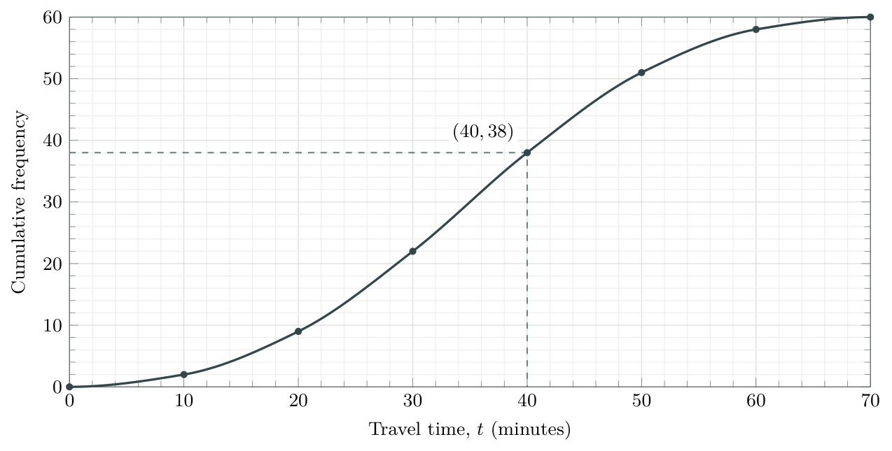
The point \((40,38)\) means 38 students travel for less than 40 minutes. Do not confuse this running total with 16, which counts only the students in \(30\le t<40\).
Final checks: the graph starts at \((0,0)\), ends at \((70,60)\) and never decreases. Its final height is \(n=60\).
Reading quartiles, percentiles and IQR
A quartile or percentile is a value of the variable, such as a travel time. To find it on a cumulative-frequency graph, first work out the number of observations that should lie below it. This count tells us where to start on the cumulative-frequency axis.
Why do we find a cumulative frequency first?
Think about the median. It marks the halfway point of the ordered data. On a grouped-data curve, we estimate it by finding the value with 50% of the observations below it.
With \(n\) observations, half of the total is \(n/2\). So we start at \(n/2\) on the vertical axis, then use the curve to find the corresponding value on the horizontal axis.
The same idea applies to the other cutoffs: the lower quartile marks 25%, the upper quartile marks 75%, and the \(p\)th percentile marks \(p\%\) of the ordered data. The graph provides estimates; repeated values can prevent an exact percentage from lying strictly below a cutoff.
Turn the required percentage into a count
The corresponding cumulative-frequency levels are \[Q_1:\ \frac n4,\qquad \text{median}:\ \frac n2,\qquad Q_3:\ \frac{3n}{4},\qquad P_p:\ \frac p{100}n.\] These are counts, not the quartile or percentile values themselves.
Find the required cumulative frequency using the total number of observations, \(n\).
Start at that count on the vertical axis and go across to the curve.
Go down to the horizontal axis. Read the variable’s value and include its units.
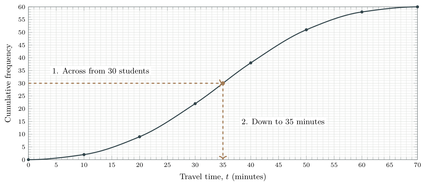
For example, with 60 travel times: half of 60 is 30, so start at cumulative frequency 30 to find the median. The curve below leads from 30 students to a travel time of approximately 35 minutes.
The count and the answer are different quantities
Here, 30 is the cumulative-frequency level used to locate the median; 35 minutes is the estimated median travel time. Do not give 30 minutes simply because \(n/2=30\).
Worked example 4: quartiles and a percentile
The table summarizes the travel times of 60 students. The row Travel time below (min) lists the time cutoffs: \(10,20,\ldots,70\) are the upper boundaries of \(0\le t<10,\ 10\le t<20,\ldots,60\le t<70\). The extra 0 is the first class’s lower boundary and supplies the starting point \((0,0)\).
| Travel time below (min) | 0 | 10 | 20 | 30 | 40 | 50 | 60 | 70 |
|---|---|---|---|---|---|---|---|---|
| Cumulative frequency | 0 | 2 | 9 | 22 | 38 | 51 | 58 | 60 |
Read each column downward. For example, 40 is the upper boundary of \(30\le t<40\); the 38 beneath it counts all students with \(t<40\), including those in earlier classes.
Use the curve below to estimate the following. Read times to the nearest minute.
the lower quartile;
the median;
the upper quartile;
the IQR;
the 80th percentile.
Step-by-step solution
Solution
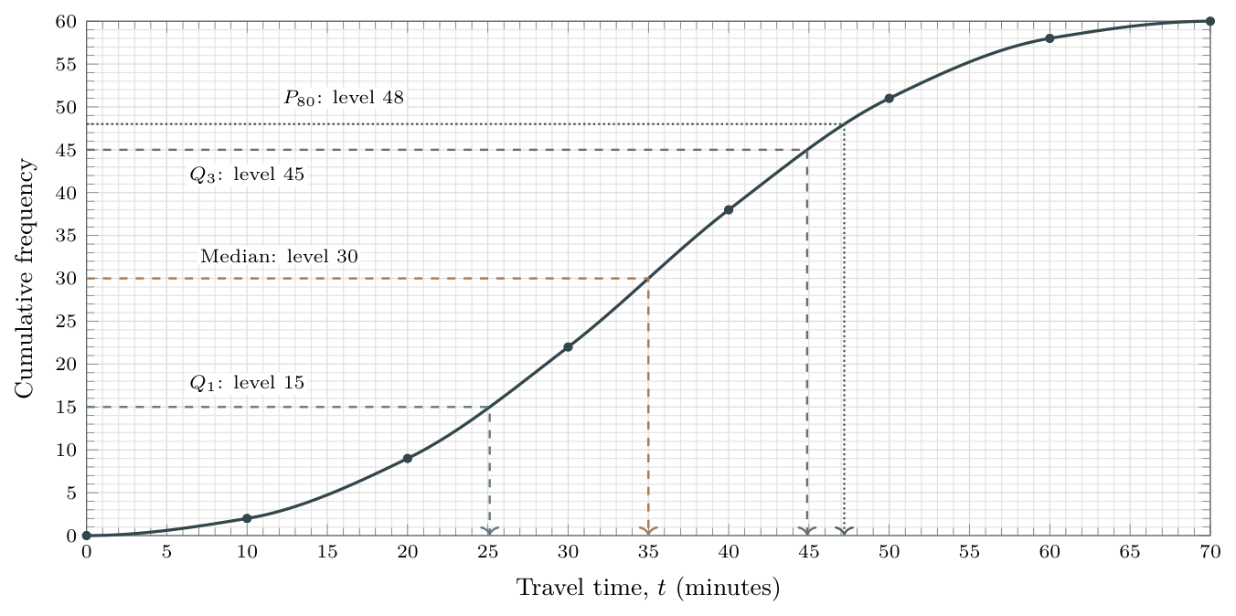
Read the grid: each small horizontal division is 1 minute; each small vertical division is 1 student.
(a) Lower quartile: at \(60/4=15\), read \(\boxed{Q_1\approx25\text{ min}}\).
(b) Median: at \(60/2=30\), read \(\boxed{\text{median}\approx35\text{ min}}\).
(c) Upper quartile: at \(3(60)/4=45\), read \(\boxed{Q_3\approx45\text{ min}}\).
(d) IQR: using these readings, \(45-25=\boxed{20\text{ min}}\) approximately.
(e) 80th percentile: at \(0.80(60)=48\), read \(\boxed{P_{80}\approx47\text{ min}}\).
These are graphical estimates, not exact data values. Use the requested accuracy and the graph’s scale; do not add decimal places that you cannot justify from the diagram.
Read the scale: a close-up
The scale tells you what a small division means
Read two labelled values and count the equal spaces between them. On the enlarged horizontal axis below, 20 to 30 minutes spans ten divisions, so each division represents 1 minute.
Worked example 5: follow a lower-quartile reading
A cumulative-frequency curve represents 60 travel times. The enlarged part of the curve below includes \((20,9)\) and \((30,22)\).
Find the cumulative-frequency level for \(Q_1\).
Use the curve to estimate \(Q_1\) to the nearest minute.
Step-by-step solution
Solution
(a) Find the level on the vertical axis
The lower-quartile level is \(60/4=15\) students. This is a count, not the time we are trying to find.
(b) Read across, then down
Start at 15 on the vertical axis. Draw a horizontal guide to the curve, then a vertical guide down to the time axis.
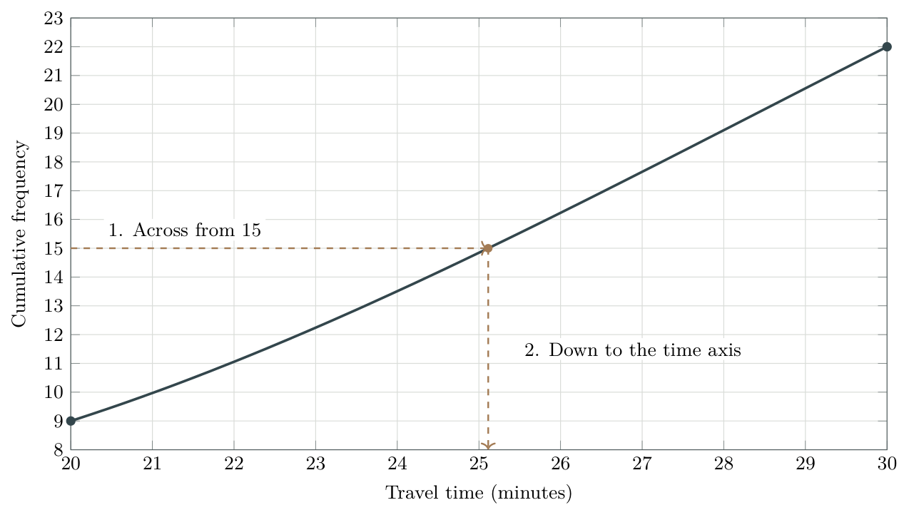
The vertical guide reaches the axis very close to 25 minutes. To the requested nearest minute, \[\boxed{Q_1\approx25\text{ minutes}}.\] Approximately one quarter of the students have travel times at or below 25 minutes. The curve does not recover the unknown individual times inside each class.
IB-style walkthrough C: cumulative frequency
[11 marks]
The heights \(h\), in centimetres, of 80 plants are grouped below.
| \(h\) (cm) | \(0\le h<10\) | \(10\le h<20\) | \(20\le h<30\) | \(30\le h<40\) | \(40\le h<50\) |
|---|---|---|---|---|---|
| Frequency | 8 | 12 | 28 | 24 | 8 |
Construct a cumulative-frequency table.[2]
Draw a cumulative-frequency graph using a smooth curve through the points.[3]
Use the graph to estimate the median and the IQR.[4]
Estimate the 90th percentile.[2]
Step-by-step solution
Solution
(a) Running totals
| Height below (cm) | 0 | 10 | 20 | 30 | 40 | 50 |
|---|---|---|---|---|---|---|
| Cumulative frequency | 0 | 8 | 20 | 48 | 72 | 80 |
The zero column is the initial lower boundary. Every other column pairs a class upper boundary with its cumulative frequency.
(b) Graph
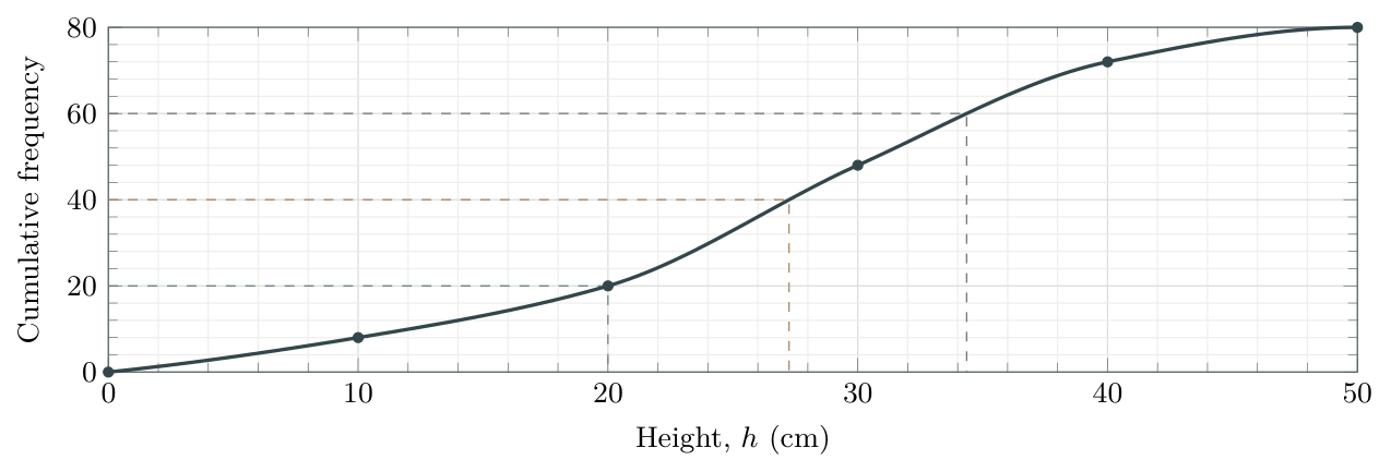
Plot \((0,0)\), \((10,8)\), \((20,20)\), \((30,48)\), \((40,72)\), \((50,80)\) and join them with a smooth, non-decreasing curve.
(c) Median and IQR
At cumulative frequency \(80/2=40\), read a median of approximately \(\boxed{27\text{ cm}}\). Read at \(80/4=20\) and \(3(80)/4=60\): \(Q_1\approx20\) cm and \(Q_3\approx34\) cm, to the nearest centimetre on this curve. \[\operatorname{IQR}\approx34-20=\boxed{14\text{ cm}}.\] Slightly different estimates are possible from a different carefully drawn curve; show the reading lines.
(d) 90th percentile
The level is \(0.90(80)=72\). The point \((40,72)\) gives \(\boxed{P_{90}\approx40\text{ cm}}\).
Keep counts and measurements separate
The median level is 40 plants; the median height is about 27 centimetres. For a quartile or percentile value, finish on the horizontal axis. When a height or time is given instead, start on that axis and read the cumulative count vertically, as in the next section.
Read from a time to a count, percentage or probability
The other direction: up to the curve, then across
When a time is given, start on the horizontal axis. Go up to the curve, then across to the left to read the cumulative frequency. This is a number of students, not a percentage. The final height gives the total, \(n\).
Worked example 6: from a graph reading to a percentage
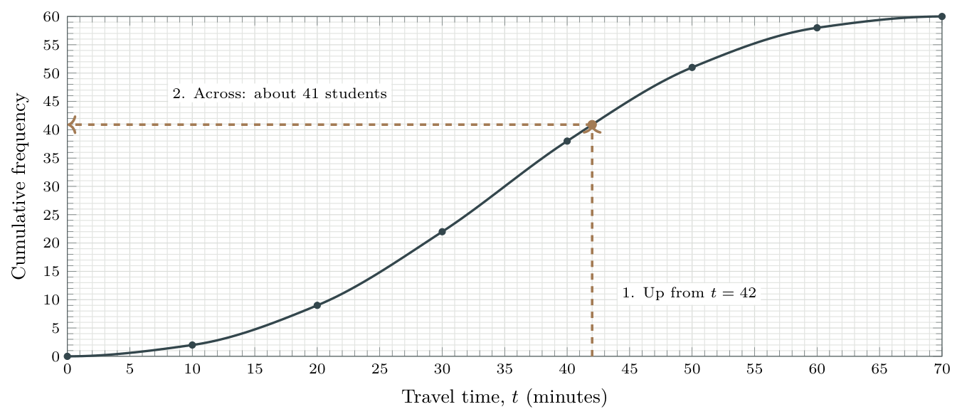
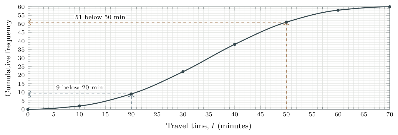
The smooth cumulative-frequency curve below represents travel times \(t\), in minutes, for 60 students. Its boundary values are listed in the table. Read intermediate counts to the nearest student.
| Travel time below (min) | 0 | 10 | 20 | 30 | 40 | 50 | 60 | 70 |
|---|---|---|---|---|---|---|---|---|
| Cumulative frequency | 0 | 2 | 9 | 22 | 38 | 51 | 58 | 60 |
Estimate how many students travel for less than 42 minutes.
Hence estimate the percentage who travel for less than 42 minutes.
One of these 60 students is selected at random, each equally likely. Estimate the probability that this student’s travel time is less than 42 minutes.
Find the number travelling for at least 50 minutes.
Find the number whose travel time satisfies \(20\le t<50\).
Recover the ordinary frequency in the class \(30\le t<40\).
Step-by-step solution
Solution
(a) Read the number of students
Locate 42, two small divisions to the right of 40. Follow the vertical guide up to the curve. Now follow the horizontal guide left: the reading is just above 40, giving \(\boxed{41\text{ students approximately}}\).
(b) Convert the count to a percentage
About 41 out of 60 students meet the condition. Divide by the total, then multiply by 100: \[\text{percentage}\approx\frac{41}{60}\times100\%\approx\boxed{68\%}.\]
(c) Convert the same count to a probability
Each of the 60 students is equally likely to be chosen, so use the same fraction, without multiplying by 100: \[\text{probability}\approx\frac{41}{60}\approx\boxed{0.68}.\] The count is a graph estimate, so the percentage and probability are estimates too. 41 is a count; 68% is a percentage; 0.68 is a probability.
(d) At least 50 minutes: remove those below 50
From 50 on the horizontal axis, go up to the curve and across: 51 students are below 50 minutes. Everyone else travels for at least 50 minutes, including exactly 50: \[\text{number at least 50}=60-51=\boxed{9\text{ students}}.\]
(e) Between 20 and 50 minutes: subtract the earlier running total
Read 51 below 50 minutes and 9 below 20 minutes. The first count includes the second. Remove those below 20, leaving exactly those with \(20\le t<50\): \[\text{number with }20\le t<50=51-9=\boxed{42\text{ students}}.\]
(f) One class: find the increase in cumulative frequency
There are 38 students below 40 minutes and 22 below 30 minutes. The increase is the number in the class \(30\le t<40\): \[\text{class frequency}=38-22=\boxed{16\text{ students}}.\] These boundary counts are given in the table, so (d)–(f) are exact for this dataset. The reading at 42 minutes was between boundaries, so (a)–(c) are estimates.
The curve is steeper where more observations occur in an equal-width interval, and flatter where fewer occur. It need not be a straight line or have one fixed shape.
Choose the direction from the wording
A percentile is given: start with a count on the vertical axis; go across, then down to the time.
A time is given: start on the horizontal axis; go up, then left to the count. To obtain a percentage or probability, divide by \(n\); multiply by 100 only for a percentage.
IB-style walkthrough D: thresholds and percentages
[9 marks]
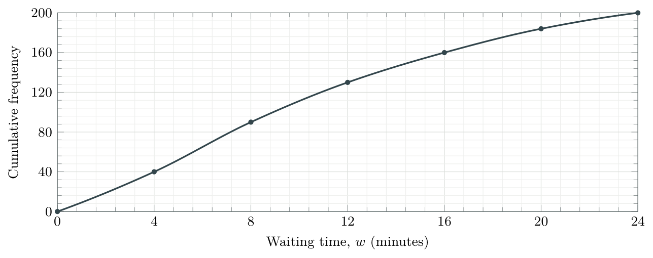
The cumulative-frequency graph shows waiting times \(w\) (minutes) for 200 customers. The marked points are \((0,0)\), \((4,40)\), \((8,90)\), \((12,130)\), \((16,160)\), \((20,184)\), \((24,200)\).
Estimate the percentage who waited less than 12 minutes.[2]
Determine the percentile rank of a waiting time of 20 minutes.[2]
Interpret your answer to part (b) in context.[1]
Estimate the number who waited at least 20 minutes.[2]
Estimate the number who waited at least 12 but less than 20 minutes.[2]
Step-by-step solution
Solution
(a) Percentage below 12
Start at 12 minutes, go up to the curve and left to read 130 customers. The graph ends at \(n=200\), so \(\frac{130}{200}\times100\%=\boxed{65\%}\).
(b) Percentile rank of 20
Go up from 20 minutes and left: 184 customers are below this time. Since \(\frac{184}{200}\times100\%=92\%\), 20 minutes is approximately the 92nd percentile.
(c) Interpretation
Approximately 92% of the customers waited less than 20 minutes. The percentage refers to customers, not a percentage of 20 minutes.
(d) At least 20
Subtract the count below 20 from the total: \(200-184=\boxed{16\text{ customers}}\).
(e) Between the thresholds
Subtract the two cumulative counts: \(184-130=\boxed{54\text{ customers}}\).
Reverse the wording, not the axes
A value exceeded by 10% is the 90th percentile: 90% are at or below it. Start at cumulative frequency \(0.90n\), not \(0.10n\), then read the value on the horizontal axis.
Box-and-whisker diagrams
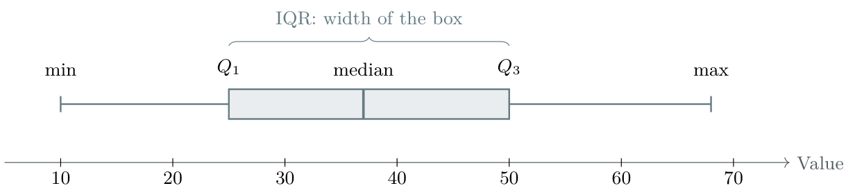
A box plot summarizes position and spread on a single numerical scale. An ordinary box plot uses \[\text{minimum},\quad Q_1,\quad \text{median},\quad Q_3,\quad \text{maximum}.\] The box runs from \(Q_1\) to \(Q_3\), with a line at the median. The whiskers extend to the extremes when there are no outliers. Outlier-adjusted whiskers are treated in 5.3 Outliers and modified box plots.
Worked example 7: draw a box plot from a summary
A dataset has minimum 12, \(Q_1=18\), median 24, \(Q_3=31\) and maximum 45. There are no outliers.
Draw a box plot.
Find the range.
Find the IQR.
Step-by-step solution
Solution
(a) Diagram
Choose a uniform scale. Draw the box from 18 to 31, median line at 24, and whiskers ending at 12 and 45.

(b) Range
\(45-12=\boxed{33}\).
(c) Interquartile range
\(31-18=\boxed{13}\).
Reading proportions, not heights
Quartiles partition the ordered data into approximately four equal groups. The box represents the middle 50%. A longer section means more spread, not more observations. With ties or small datasets, do not insist that exactly 25% lie strictly between each pair of numerical cutoffs. The box’s vertical height has no statistical meaning.
Deducing missing values in a box plot
Turn the information into an equation
Use \(\text{range}=\text{maximum}-\text{minimum}\) and \(\operatorname{IQR}=Q_3-Q_1\). Substitute the known values, then solve for the missing one. Use any extra condition about the median only when it is stated.
Worked example 8: recover three missing summary values [8 marks]
The incomplete five-number summary below describes a set of test scores. There are no outliers.
| Minimum | \(Q_1\) | Median | \(Q_3\) | Maximum |
|---|---|---|---|---|
| \(a\) | 20 | \(b\) | \(c\) | 58 |
The range is 48 and the IQR is 24. The median lies exactly halfway between \(Q_1\) and \(Q_3\).
Find the minimum, \(a\).[2]
Find the upper quartile, \(c\).[2]
Hence find the median, \(b\).[2]
Draw the completed box plot on a labelled numerical scale.[2]
Step-by-step solution
Solution
(a) Use the range to find the minimum
The maximum is 58 and the full spread is 48, so \[48=58-a\quad\Rightarrow\quad a=58-48=\boxed{10}.\]
(b) Use the IQR to find the upper quartile
The box starts at \(Q_1=20\) and has width 24, so \[24=c-20\quad\Rightarrow\quad c=20+24=\boxed{44}.\]
(c) Use the stated position of the median
We are told that the median is halfway between the quartiles. Therefore \[b=\frac{20+44}{2}=\boxed{32}.\]
(d) Construct the completed plot
The five-number summary is \(10,20,32,44,58\). Draw whiskers ending at 10 and 58, the box from 20 to 44, and the median line at 32.

Check: \(58-10=48\) and \(44-20=24\), as required. The values are in increasing order.
The median need not be the midpoint of the box
Here the midpoint calculation is justified by the question. Without that extra condition, the range and IQR alone would not determine the median. Do not assume a box plot is symmetric.
From cumulative frequency to a box plot
A class boundary is not an observed extreme
The start \((0,0)\) of a grouped-data graph does not prove that the smallest observed value is 0. Likewise, \((70,60)\) does not prove that the maximum is 70. If only those class boundaries are known, the exact range cannot be recovered. Their difference, 70, is only a boundary-based approximation when such an estimate is requested.
Worked example 9: link the two representations
The travel times (minutes) of 60 students have this cumulative-frequency table. The actual shortest and longest journeys were 3 and 67 minutes. No outliers were identified.
| Travel time below (min) | 0 | 10 | 20 | 30 | 40 | 50 | 60 | 70 |
|---|---|---|---|---|---|---|---|---|
| Cumulative frequency | 0 | 2 | 9 | 22 | 38 | 51 | 58 | 60 |
Estimate \(Q_1\), the median and \(Q_3\) from the curve, to the nearest minute.
State the range and estimate the IQR.
Draw a box plot using the estimated quartiles and known extremes.
Step-by-step solution
Solution
(a) Read the three quartile levels
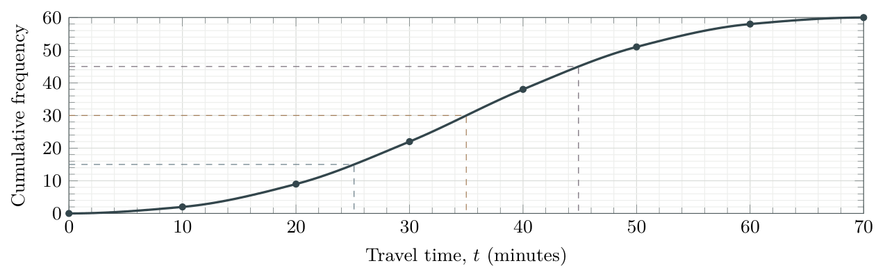
The levels are \(15,30,45\). Read \(Q_1\approx25\), median \(\approx35\) and \(Q_3\approx45\) minutes from the curve.
(b) Separate exact from estimated spread
Range \(=67-3=\boxed{64\text{ minutes}}\) exactly; IQR \(\approx45-25=\boxed{20\text{ minutes}}\).
(c) Use one common scale
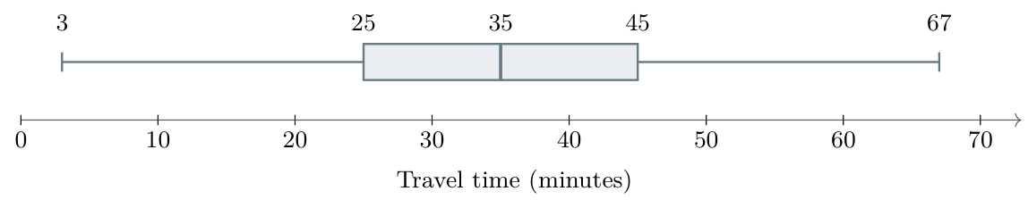
When a range reading is justified
If a question gives the actual smallest and largest observations, use them. If a graph explicitly marks the observed extremes, read those. With grouped class endpoints alone, explain that the extremes are unknown; do not silently treat class boundaries as data values.
Outliers and modified box plots
The outlier rule
An observation is an outlier if it lies strictly below \(Q_1-1.5\operatorname{IQR}\) or strictly above \(Q_3+1.5\operatorname{IQR}\). These thresholds are the fences. \[\text{Lower fence}=Q_1-1.5\operatorname{IQR},\quad \text{Upper fence}=Q_3+1.5\operatorname{IQR}.\] A value equal to a fence is not an outlier under this rule. Show outliers as crosses in an IB-style diagram. Each whisker ends at the most extreme observed non-outlier, not at the fence itself.
Worked example 10: identify and show an outlier
The ordered data are 10, 12, 13, 15, 17, 18, 20, 22, 25, 27, 28, 30, 31, 33, 36, 55. Use \(Q_1=16\), median \(23.5\) and \(Q_3=30.5\).
Calculate the IQR and both fences.
Identify any outliers.
Draw a modified box plot.
Find the range of the complete dataset.
Step-by-step solution
Solution
(a) IQR and fences
\[\begin{aligned} \operatorname{IQR}&=30.5-16=14.5,\\ \text{Lower fence}&=16-1.5(14.5)=-5.75,\\ \text{Upper fence}&=30.5+1.5(14.5)=52.25. \end{aligned}\]
(b) Outlier
\(55>52.25\), so 55 is the only outlier. No observation is below \(-5.75\).
(c) Modified box plot
The lower whisker ends at 10; the upper whisker ends at 36, the largest non-outlier.

(d) Full range
\(55-10=\boxed{45}\). The outlier remains part of the dataset; the whisker-to-whisker distance is not the full range.
Do not automatically delete an outlier
An unusual observation can be genuine. Investigate its context or a possible recording error before deciding how to handle it; identifying an outlier does not prove it is wrong.
IB-style walkthrough E: a modified box plot
[10 marks]
The ordered measurements, in centimetres, are 10, 12, 14, 16, 18, 20, 22, 24, 26, 30, 34, 60.
Use technology to determine the median, \(Q_1\) and \(Q_3\).[3]
Determine the IQR and calculate both outlier fences.[3]
Identify any outliers and construct a modified box plot.[4]
Step-by-step solution
Solution
(a) Quartiles
Enter the 12 values as a raw list with frequency 1. The calculator gives median \(21\), \(Q_1=15\) and \(Q_3=28\) cm. To check the median, average the 6th and 7th values: \[\text{median}=\frac{20+22}{2}=21\text{ cm}.\] The lower six values are \(10,12,14,16,18,20\). Their median is \[Q_1=\frac{14+16}{2}=15\text{ cm}.\] The upper six values are \(22,24,26,30,34,60\). Their median is \[Q_3=\frac{26+30}{2}=28\text{ cm}.\]
(b) IQR and fences
\[\begin{aligned} \operatorname{IQR}&=28-15=13\text{ cm},\\ \text{Lower fence}&=15-1.5(13)=-4.5\text{ cm},\\ \text{Upper fence}&=28+1.5(13)=47.5\text{ cm}. \end{aligned}\]
(c) Outlier and diagram
\(60>47.5\), so 60 cm is the only outlier. The observed non-outlier extremes are 10 cm and 34 cm. Draw the box from 15 to 28, the median at 21, and a cross at 60.

A quick self-check
The right whisker ends at 34, not 47.5 and not 60. The upper fence 47.5 is a decision threshold, not a measured value. The full data range would still be \(60-10=50\) cm.
Comparing distributions in context
Compare centre, spread, shape and unusual values
Use medians for typical values, IQRs for the spread of the middle half, and ranges for total spread. Compare shapes and outliers when relevant. Use the same numerical scale for both plots. A higher value is only “better” when the context makes it so.
Worked example 11: compare two classes’ test scores
Two classes sit the same test. Their summaries are shown below. For Class B, the lowest non-outlier is 48; its score of 18 is an outlier.
| Class | Minimum | \(Q_1\) | Median | \(Q_3\) | Maximum |
|---|---|---|---|---|---|
| A | 42 | 56 | 65 | 74 | 88 |
| B | 18 | 60 | 68 | 72 | 82 |
Compare the typical performance.
Compare the IQRs and overall ranges.
Describe the symmetry and unusual values, then write a conclusion in context.
Step-by-step solution
Solution

(a) Typical performance
Class B’s median is higher: \(68>65\). A typical score is slightly higher in Class B.
(b) Middle spread and full spread
\[\begin{aligned} \operatorname{IQR}_A&=74-56=18,&\operatorname{range}_A&=88-42=46,\\ \operatorname{IQR}_B&=72-60=12,&\operatorname{range}_B&=82-18=64. \end{aligned}\] Class B’s middle 50% is less spread out, but its full range is larger because of the low outlier.
(c) Shape, unusual values and conclusion
Class A is approximately symmetric: both halves of its box have width 9 and both whiskers have length 14. Class B is not symmetric and has an unusually low score of 18.
Conclusion: Class B typically performed slightly better and had a more consistent middle half, but its low outlier made its overall spread greater.
Two limits of a box plot
A box plot does not usually show sample size or the mean. Nor can you determine an arbitrary percentage between two values inside a quartile from the box alone. “Smaller IQR” does not mean every measure of spread is smaller.
Shape, symmetry and possible normality

Symmetry: the median is near the centre of the box and the whiskers have similar lengths. Skewness: the longer-spread side indicates the tail direction. These features suggest shape; five summary values cannot reveal every detail of a distribution.
Does symmetry suggest a normal distribution?
A normal distribution is symmetric and bell-shaped. An approximately symmetric box plot can be consistent with normality, but does not prove it: a non-normal distribution can also be symmetric. Outliers may occur in normal samples; their absence is not a requirement for normality.
IB-style walkthrough F: comparing groups [8 marks]
Two groups complete the same test. Neither has an outlier under the \(1.5\operatorname{IQR}\) rule.
| Group | Minimum | \(Q_1\) | Median | \(Q_3\) | Maximum |
|---|---|---|---|---|---|
| A | 32 | 44 | 55 | 66 | 78 |
| B | 20 | 40 | 56 | 60 | 90 |

Calculate the IQR and range for each group.[4]
Compare typical performance and consistency.[2]
Which group gives stronger evidence of symmetry? Explain why this does not prove normality.[2]
Step-by-step solution
Solution
(a) Spread
Group A: IQR \(=66-44=22\); range \(=78-32=46\).
Group B: IQR \(=60-40=20\); range \(=90-20=70\).
(b) Compare in context
The medians are similar, with B slightly higher (\(56>55\)). B’s middle half is a little less spread out, but its overall range is much larger. Do not say B is less variable in every sense.
(c) Symmetry is evidence, not proof
Group A has equal box halves (\(55-44=66-55=11\)) and equal whiskers (\(44-32=78-66=12\)). Its box plot therefore gives stronger evidence of symmetry. The data may be approximately normal, but the box plot alone cannot establish a bell-shaped distribution.
TI-Nspire CX
One-variable statistics and a box plot from raw data
Follow the written steps and compare your screen with the images below. Menu wording may vary slightly by software version; use the named options.
A. Enter the observations and run One-Variable Statistics
Use the measurements from walkthrough E: 10, 12, 14, 16, 18, 20, 22, 24, 26, 30, 34, 60.
From Home, start a New Document and choose Add Lists & Spreadsheet.
Name column A
values. Leave the grey formula row blank. Enter one observation in each numbered row, starting at row 1. There must be 12 entries.Select an empty cell in column C for the results, as in the illustrated output. Choose Menu › Statistics › Stat Calculations › One-Variable Statistics.
Set Number of Lists to 1. Set X1 List to
values; leave Frequency List as1. This means every entered observation occurs once.Keep the category fields at their defaults. Check that the first result column is empty (column C here), then select OK.
Scroll to \(n\),
MinX,Q1X,MedianX,Q3XandMaxX. Output names may appear with slightly different capitalization or spacing.
Raw-data entry
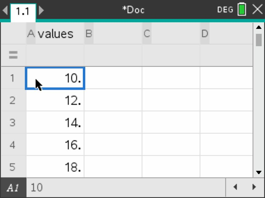
values. The first five entries are
visible; continue below to enter all 12.Five-number summary output
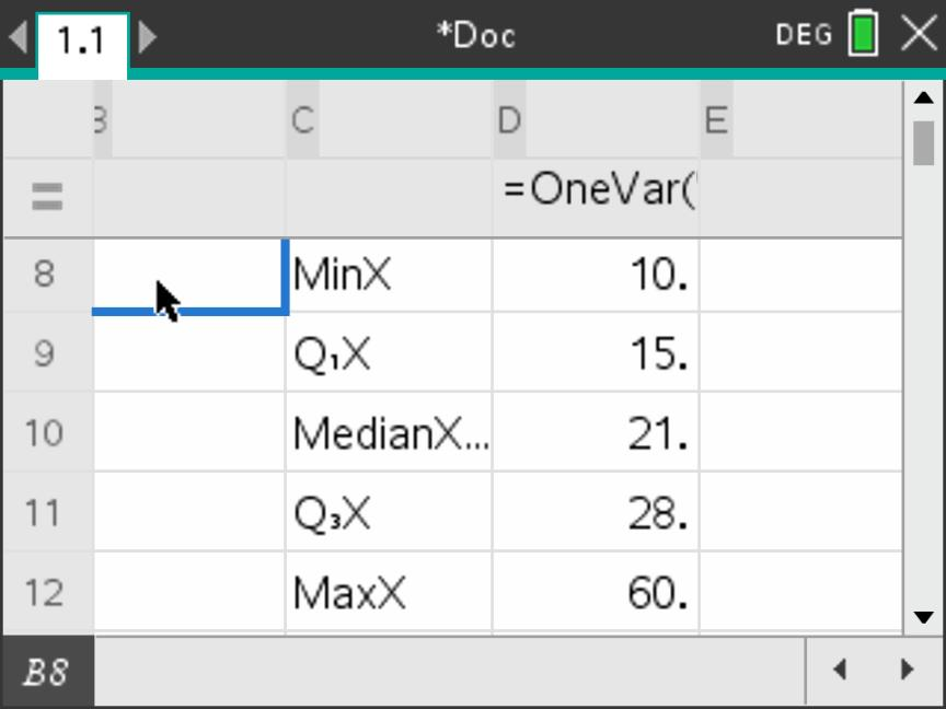
Results you should obtain
| \(n\) | Minimum | \(Q_1\) | Median | \(Q_3\) | Maximum |
|---|---|---|---|---|---|
| 12 | 10 | 15 | 21 | 28 | 60 |
\[\operatorname{IQR}=28-15=13,\qquad \text{range}=60-10=50.\] Do not confuse sx or \(\sigma_x\) with a quartile: these are standard-deviation outputs, treated in section 4.3.
B. Display the box plot
Keep the list values entered in Part A (section 7.1 One-variable statistics and a box plot from raw data) in the same problem. Follow the screenshots from left to right, then continue with the next row. The full dataset is 10, 12, 14, 16, 18, 20, 22, 24, 26, 30, 34, 60.
1. Open the Insert menu
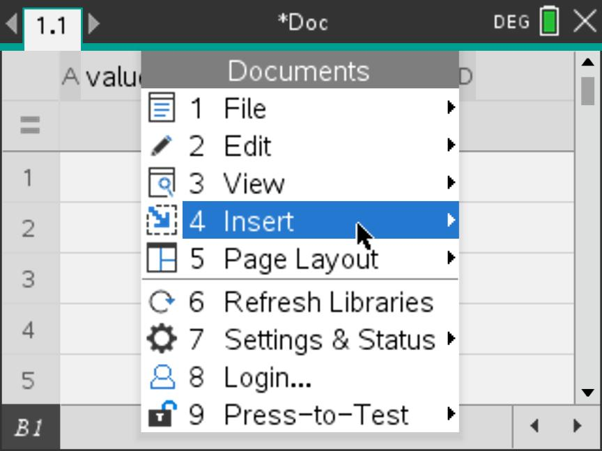
2. Add Data & Statistics
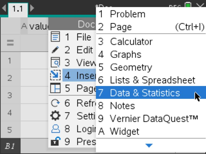
values.3. Choose the horizontal variable
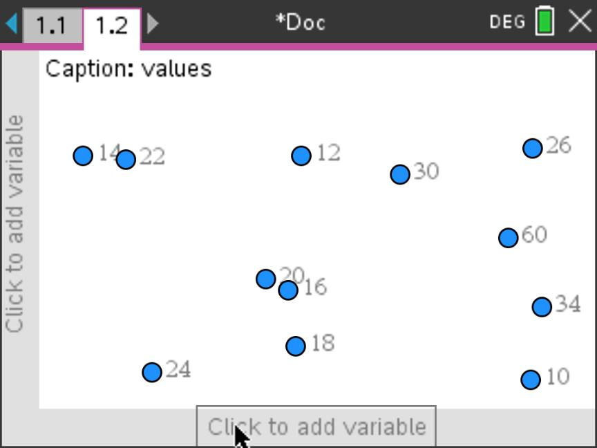
values from the list that opens. Leave
the vertical variable blank.4. Check the dot plot
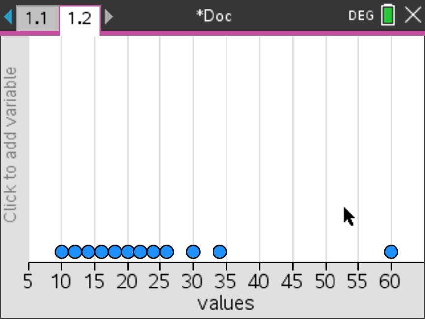
values. The separate point at 60 is part of the original
data.Why the two displays look different
In Step 3, the observations are not yet positioned on a numerical axis. Selecting values produces the dot plot in Step 4. Next, change the display type; do not change or re-enter the data.
The dot plot and box plot represent the same 12 observations. Use the next two screens to change the representation, then use Step 7 to read an exact summary value from the display.
5. Select Box Plot
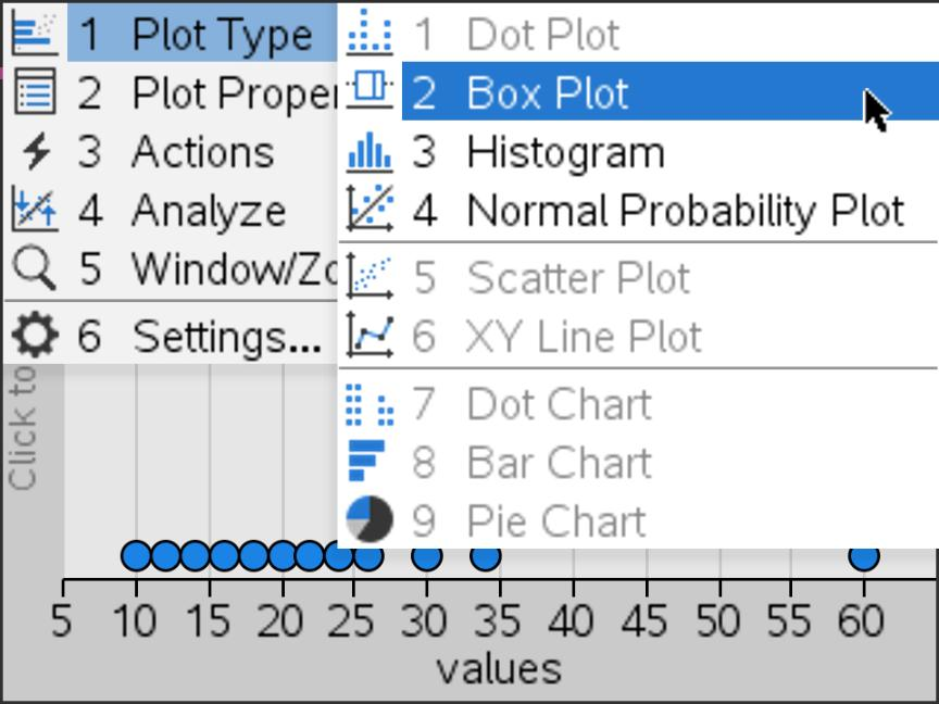
6. Inspect the modified box plot
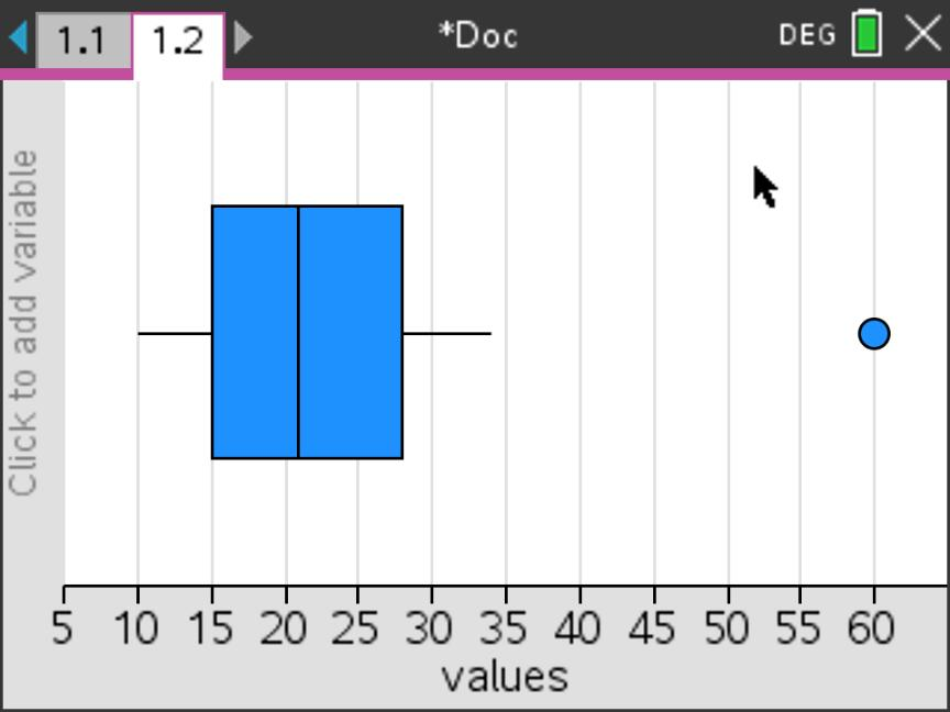
7. Read a value from the plot
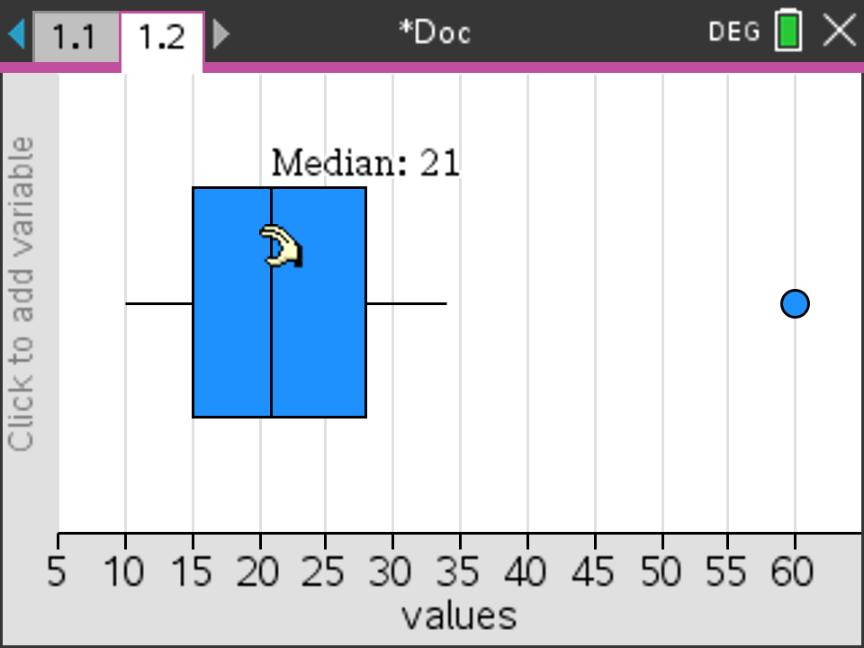
Check what each feature represents
| Feature | Value |
|---|---|
| Lower whisker | 10 |
| Left edge of the box, \(Q_1\) | 15 |
| Median line | 21 |
| Right edge of the box, \(Q_3\) | 28 |
| Upper non-outlier whisker | 34 |
| Separate outlier | 60 |
The overall maximum is still 60. The upper whisker is 34, the largest observation that is not an outlier.
Read the display; do not change the observations
Do not drag a point or part of the plot: this can change the data. The calculator shows the outlier as a dot; in your hand-drawn answer, mark it with a cross.
If the display differs: use Window/Zoom › Zoom – Data to show all the data. If the whisker extends to 60, choose Plot Properties › Show Box Plot Outliers. Analyze › Graph Trace is another way to inspect the plot’s summary values.
One-variable statistics and a box plot from a frequency table
A. Enter the data and run One-Variable Statistics
The table shows the mathematics examination grades obtained by 45 students. Grades are reported on a scale from 1 to 7.
| Grade, \(x\) | 1 | 2 | 3 | 4 | 5 | 6 | 7 |
|---|---|---|---|---|---|---|---|
| Frequency, \(f\) | 2 | 1 | 5 | 9 | 12 | 9 | 7 |
Use the data to find the minimum, lower quartile, median, upper quartile and maximum. Then display a box plot in Part B.
Read the table first. The frequency 12 below grade 5 means that 12 students obtained grade 5. The frequencies are counts, not additional grades.
1. Enter the grades and frequencies
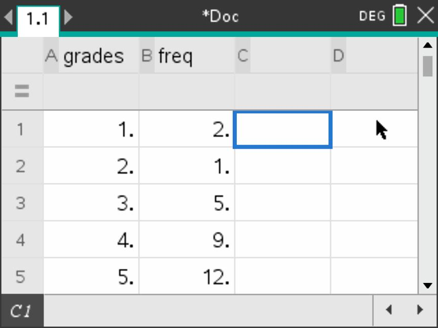
grades and column B
freq. Leave the grey formula row blank. Enter each grade
and its frequency on the same numbered row. The first
five pairs are visible; also enter \((6,9)\) and \((7,7)\) below them.2. Open One-Variable Statistics
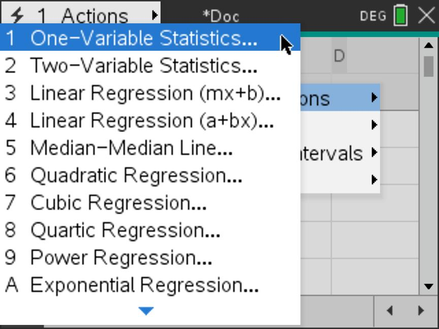
Seven categories, but 45 observations
\[n=2+1+5+9+12+9+7=45.\] There are seven different grades but 45 students. Do not enter 45 as an eighth row: it is the total frequency, not another grade. When calculating the statistics, the calculator must use freq to count each grade the correct number of times.
Continue with the setup on the next steps below. The list names grades and freq match the supplied screens throughout this example.
Continue with the two lists from section 7.2 One-variable statistics and a box plot from a frequency table. Follow the screens from left to right, then move to the next row. The essential choice is X1 List = grades and Frequency List = freq.
3. Choose one variable
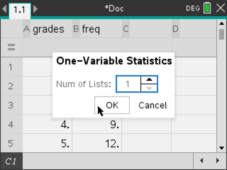
4. Select the data list
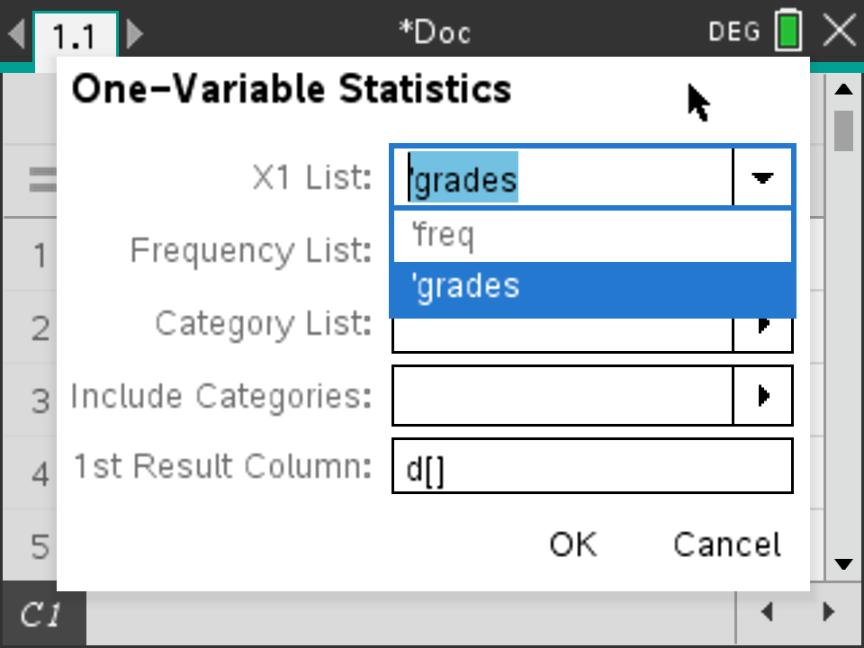
grades. This tells the calculator which numbers are the
observed values. Do not select freq here: those numbers are
counts of students.5. Select the frequency list
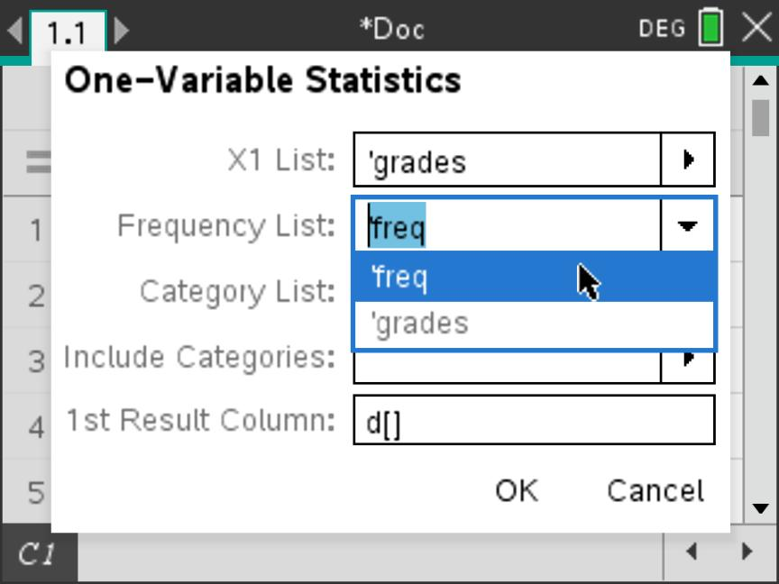
freq. This tells the calculator that grade 1 occurs twice,
grade 2 once, grade 3 five times, and so on. Do not
leave this field as 1 for these data.6. Confirm the setup and calculate
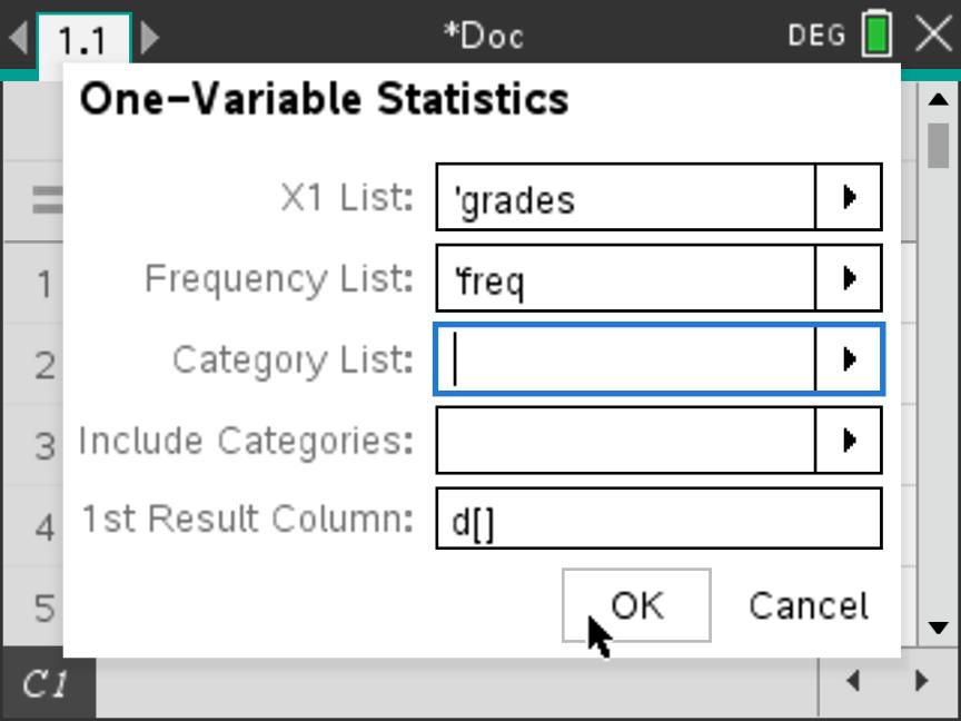
d[] as the 1st Result Column,
so the output appears in D–E. Select OK.Use the counts, not just the seven grade labels
Leaving Frequency List = 1 treats each of \(1,2,\ldots,7\) as occurring once. That would describe only seven students and give median 4, not the intended distribution of 45 students.
Scroll to the five-number summary. The values below are summaries of the 45 students’ grades, with every grade counted according to its frequency.
7. Read the five-number summary
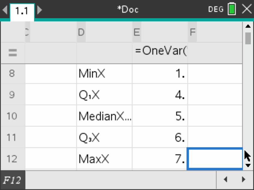
MinX, \(Q_1\), the
median, \(Q_3\) and MaxX.
Scroll upwards separately to check \(n=45\); that row is not visible in this
image.Results you should obtain
| Measure | Value |
|---|---|
| Minimum | 1 |
| Lower quartile, \(Q_1\) | 4 |
| Median | 5 |
| Upper quartile, \(Q_3\) | 6 |
| Maximum | 7 |
IQR: \(6-4=2\) grades.
Range: \(7-1=6\) grades.
Mode: grade 5, since its frequency, 12, is the largest in the original table. Find the mode from that table, not from this output.
B. Display the box plot
Keep grades and freq in the same problem. The plot must also use the frequencies: calculating the statistics does not automatically apply those counts to a new plot. Follow the screens from left to right.
1. Open Summary Plot
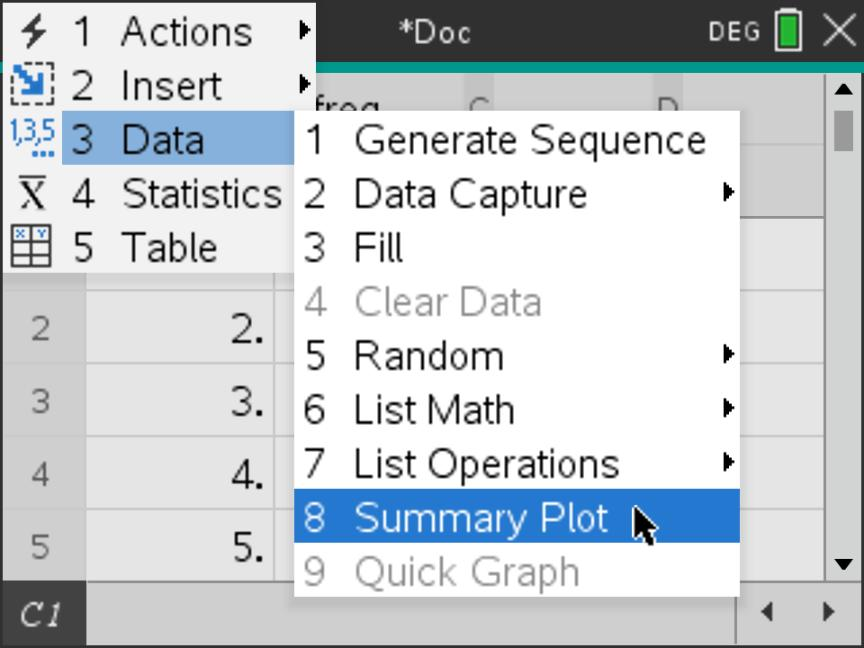
2. Link the values to their counts
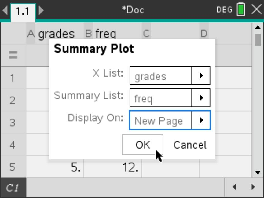
grades, Summary
List = freq and Display On = New
Page. Check both list names, then select OK.
Grade 5 will be counted 12 times, not just once.Continue on the next steps below: the initial display may be a histogram. Keep the same data and change its plot type to a box plot.
The histogram and box plot below represent the same 45 students. Only the display changes. Follow Steps 3–6 without re-entering the data or removing the frequency list.
3. Recognise the initial histogram
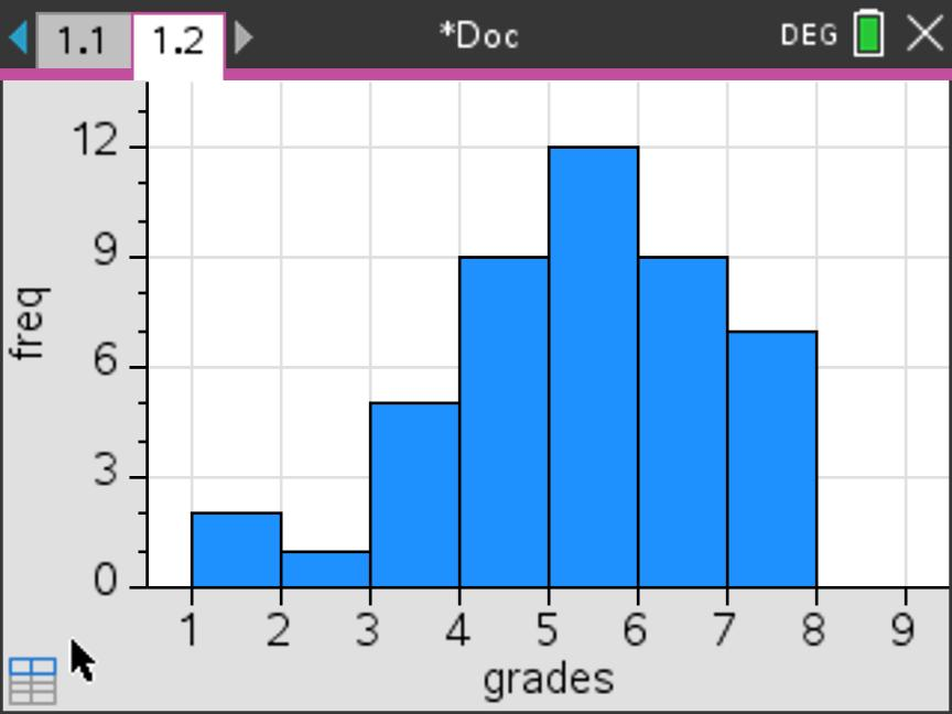
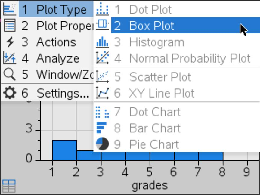
4. Change the plot type to Box Plot
grades and freq association. The same
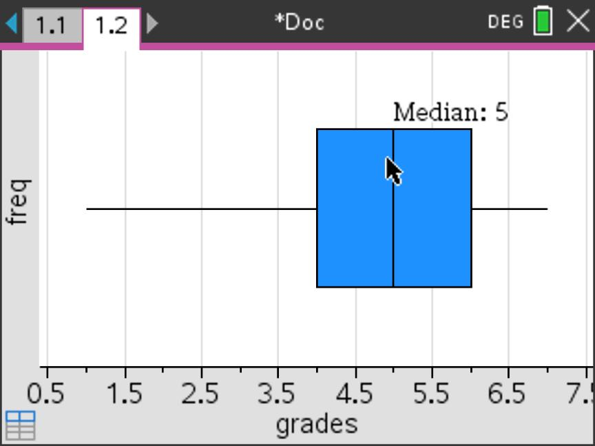
observations are now shown as a box-and-whisker diagram.5. Read the median directly
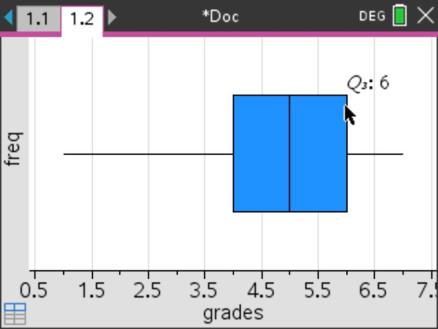
6. Read the upper quartile directly
freq label is not a vertical scale:
read summary values from their horizontal
positions.Check the frequencies were retained
The five-number summary is 1, 4, 5, 6, 7, matching Part A. If the median is 4 instead of 5, the seven grade labels may have been plotted without their frequencies; return to Summary Plot and check Summary List = freq.
Here \(\operatorname{IQR}=6-4=2\). The outlier fences are \(4-1.5(2)=1\) and \(6+1.5(2)=9\). Grade 1 lies on the lower fence, so it is not an outlier; both whiskers reach the actual minimum and maximum.
An equal-width grouped histogram
A. Start with the original grouped data
A researcher records the time \(t\), in minutes, taken by 40 students to complete a task. These are the grouped data from walkthrough B.
| Time, \(t\) (min) | \(0\le t<10\) | \(10\le t<20\) | \(20\le t<30\) | \(30\le t<40\) | \(40\le t<50\) |
|---|---|---|---|---|---|
| Frequency, \(f\) | 4 | 10 | 14 | 8 | 4 |
The exact individual times are not given. To enter these grouped data for the histogram, use one midpoint to represent each class, paired with that class’s frequency.
B. Find the class midpoints, then prepare the frequency table
The midpoint (or mid-value) lies halfway between the two class boundaries. Add the boundaries and divide by 2: \[\boxed{\text{Class midpoint}=\frac{\text{lower boundary}+\text{upper boundary}}{2}.}\] For example, the midpoint of \(20\le t<30\) is \((20+30)/2=25\) minutes. Applying the same method to every class gives:
| Calculation | \(\dfrac{0+10}{2}\) | \(\dfrac{10+20}{2}\) | \(\dfrac{20+30}{2}\) | \(\dfrac{30+40}{2}\) | \(\dfrac{40+50}{2}\) |
|---|---|---|---|---|---|
| Midpoint, \(m\) (min) | 5 | 15 | 25 | 35 | 45 |
| Frequency, \(f\) | 4 | 10 | 14 | 8 | 4 |
Keep the frequencies unchanged. The midpoint 25 is paired with 14 because 14 students are in \(20\le t<30\); this does not mean that all 14 took exactly 25 minutes.
Representatives only. Do not treat these midpoints as the exact raw-data minimum, maximum or quartiles. Use the cumulative-frequency methods in Sections 3–4 to estimate grouped-data quartiles.
C. Enter the lists and open Summary Plot
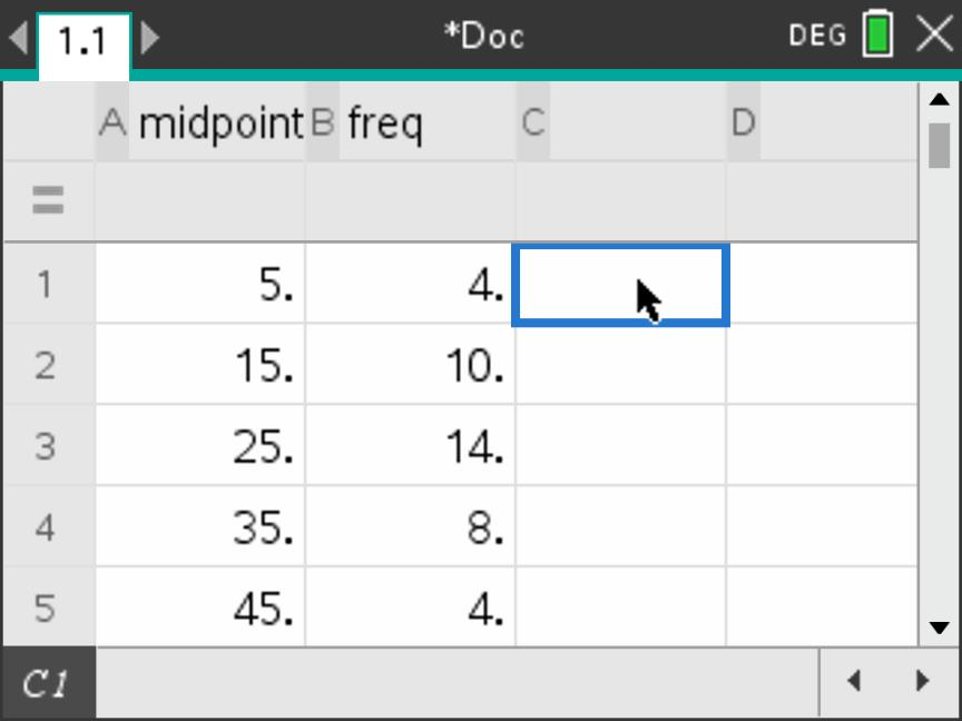
Start a new problem and add Lists & Spreadsheet. Name column A midpoint and column B freq. Leave the grey formula row blank. Enter the five pairs \((5,4)\), \((15,10)\), \((25,14)\), \((35,8)\) and \((45,4)\), starting in row 1.
1. Check the paired entries
2. Open Summary Plot
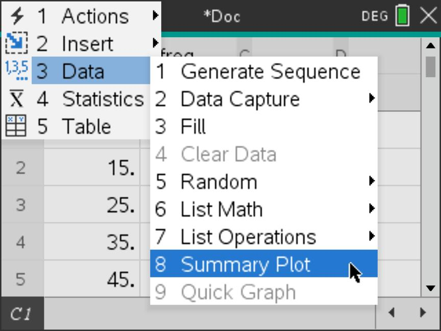
The midpoint list is \((5,15,25,35,45)\) and freq is \((4,10,14,8,4)\). Select both lists in the dialog so that the histogram uses all 40 students, rather than counting each midpoint once.
3. Link midpoints to frequencies
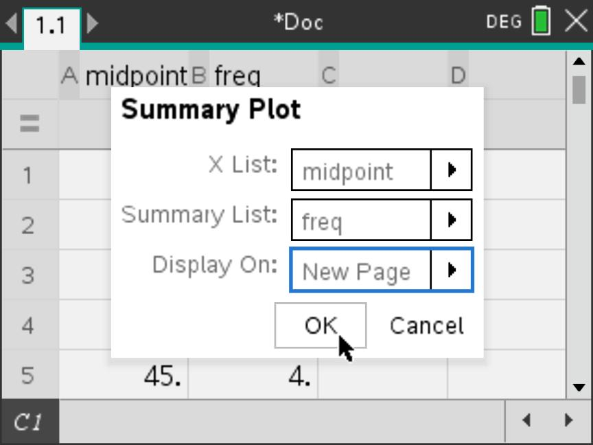
midpoint, Summary
List = freq and Display On = New
Page. Select OK.4. Recognise the initial histogram
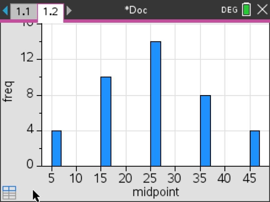
D. Match the bins to the original class intervals
A bin is a histogram class interval. Our classes are \(0\le t<10\), \(10\le t<20\), and so on. The histogram therefore needs a width of 10 and boundaries aligned at 0, 10, 20, 30, 40 and 50.
5. Open Histogram Properties
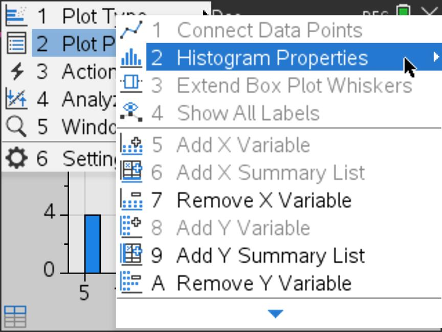
6. Choose Equal Bin Width
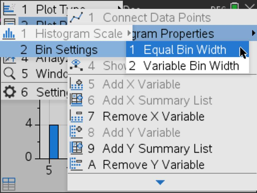
Do not interpret the initial gaps as gaps in the original data
The first display uses the entered midpoints with automatic bins. The empty spaces in Step 4 do not show that no students took the intervening times. Set the bins to the original class intervals before interpreting the grouped distribution.
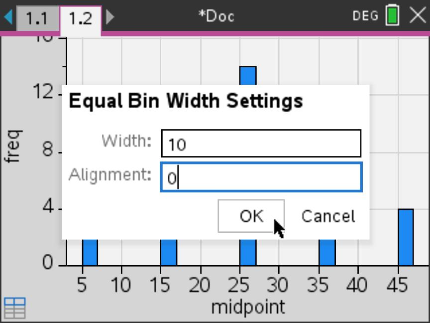
Width = 10 makes every class ten minutes wide. Alignment = 0 places a boundary at zero, so the next boundaries occur at \(10,20,30,40\) and \(50\). Keep the vertical scale as Frequency; no density calculation is needed.
7. Apply the width and alignment
8. Inspect the complete histogram
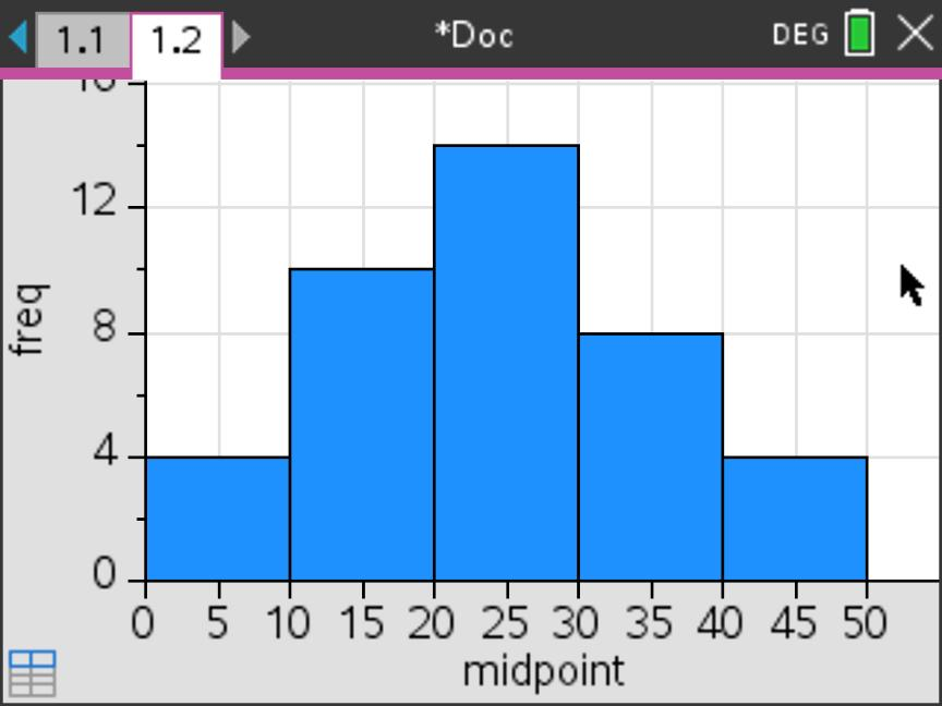
Read the class boundaries
The screen labels the horizontal axis every 5 minutes, but each bar spans 10 minutes. Read the class boundaries at \(0,10,20,30,40,50\), not at every tick mark. For example, the tallest bar extends from 20 to 30 minutes and has frequency 14.
. Check against the complete histogram
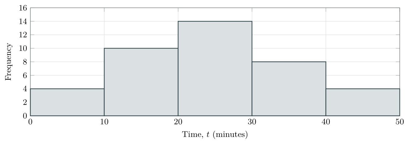
Read the result. The tallest bar spans \(20\le t<30\) and represents 14 students. Adding the five heights gives \(4+10+14+8+4=\boxed{40}\) students. The calculator’s horizontal label midpoint is the list name; on paper label the original variable time (minutes) and mark the class boundaries, as above.
Calculator reference. The supplied screenshots illustrate the procedures. Summary Plot defaults, bin settings and window controls were checked against Texas Instruments’ TI-Nspire Technology eGuide. Source links are included in the package.
Independent mastery practice — new data
Work without the solutions first
Use a graphical calculator for statistical summaries. Show the relevant values, calculations and interpretations; calculator output alone is not a complete explanation. Draw graphs on squared paper and show reading lines. For cumulative-frequency diagrams, use a smooth curve through the points. Give times to the nearest whole minute or second unless stated otherwise. The worked answers use the stated median-of-halves convention or matching TI-Nspire output. Answers begin in 9. Answer key and solution outlines.
1. Data and class boundaries.
Classify each variable as discrete or continuous: number of late arrivals; mass of a parcel; time taken to run 100 metres.
The classes are \(0\le t<10\), \(10\le t<20\), \(20\le t<30\). Where does \(t=20\) belong? Give the class width.
State one suitable graphical display for the running times and explain why it is suitable.
Show the full answer
Solution
(a) Types
Late-arrival count: discrete. Parcel mass and running time: continuous.
(b) Boundary
\(t=20\) belongs to \(20\le t<30\); width \(=30-20=10\).
(c) Suitable graph
A histogram displays the grouped distribution of running times on a numerical scale. A cumulative-frequency graph is also suitable when the aim is to read percentages or percentile times.
2. A discrete frequency distribution.
The numbers of puzzles completed by 12 students are 0, 1, 1, 2, 2, 2, 3, 3, 4, 4, 4, 4.
Construct a frequency table and verify its total.
Find the mode.
Find the percentage who completed at least three puzzles.
Show the full answer
Solution
(a) Table
| Puzzles | 0 | 1 | 2 | 3 | 4 | Total |
|---|---|---|---|---|---|---|
| Frequency | 1 | 2 | 3 | 2 | 4 | 12 |
(b) Mode
4 puzzles: this value has the greatest frequency, 4.
(c) Percentage
At least three puzzles: \(2+4=6\) students. \(\frac6{12}\times100\%=50\%\).
3. Raw-data quartiles.
The eight values are \(15,4,10,7,19,6,13,11\). Use technology for the summary measures.
Write them in ascending order.
Find the median, \(Q_1\) and \(Q_3\).
Find the range and IQR.
Show the full answer
Solution
(a) Order
\(4,6,7,10,11,13,15,19\).
(b) Centre and quartiles
Median \(=(10+11)/2=10.5\); \(Q_1=(6+7)/2=6.5\); \(Q_3=(13+15)/2=14\).
(c) Spread
Range \(=19-4=15\); IQR \(=14-6.5=7.5\).
4. A clinic’s waiting times.
| \(t\) (min) | \(0\le t<10\) | \(10\le t<20\) | \(20\le t<30\) | \(30\le t<40\) | \(40\le t<50\) | \(50\le t<60\) |
|---|---|---|---|---|---|---|
| Frequency | 3 | 7 | 12 | 9 | 6 | 3 |
Draw a frequency histogram and state the modal class.
Find the number of patients with \(10\le t<40\).
Find the percentage with \(t<30\).
Show the full answer
Solution
(a) Histogram and modal class
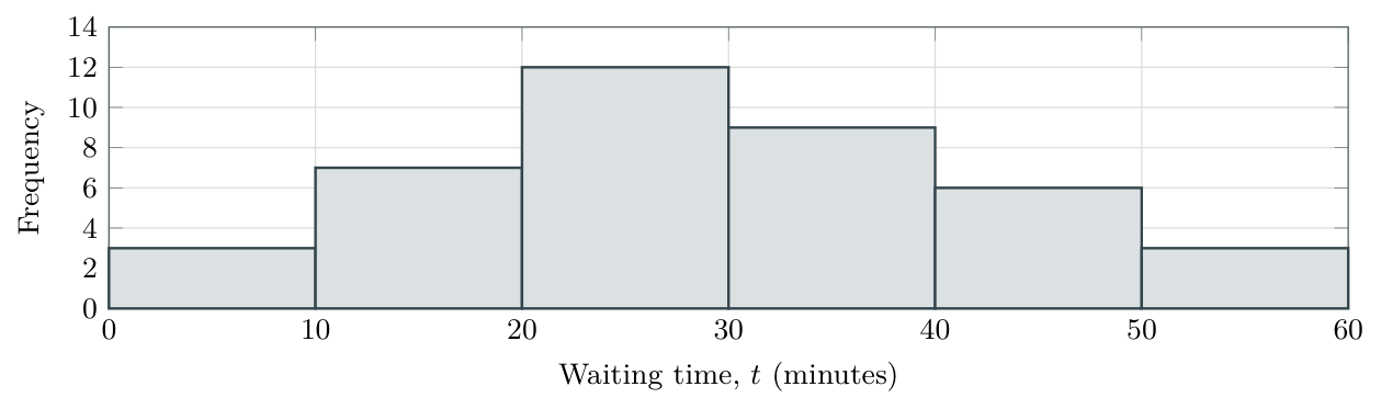
The modal class is \(20\le t<30\) minutes. All six rectangles occupy intervals of width 10.
(b) Number
\(7+12+9=28\) patients have \(10\le t<40\).
(c) Percentage
There are \(n=40\) patients; \(3+7+12=22\) have \(t<30\). \(\frac{22}{40}\times100\%=55\%\).
5. Cumulative frequency for the clinic.
The frequencies in the consecutive intervals \(0\le t<10\), \(10\le t<20\), \(20\le t<30\), \(30\le t<40\), \(40\le t<50\), \(50\le t<60\) are \(3,7,12,9,6,3\).
Construct a cumulative-frequency table and graph.
Estimate \(Q_1\), the median, \(Q_3\) and the IQR.
Estimate \(P_{90}\) and interpret it in context.
Show the full answer
Solution
(a) Table and graph
| Waiting time below (min) | 0 | 10 | 20 | 30 | 40 | 50 | 60 |
|---|---|---|---|---|---|---|---|
| Cumulative frequency | 0 | 3 | 10 | 22 | 31 | 37 | 40 |
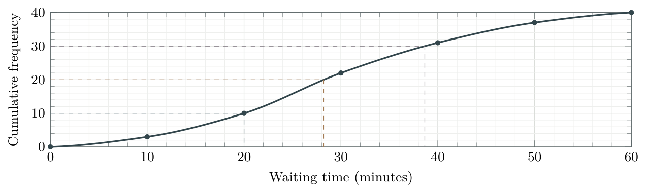
(b) Quartiles and IQR
With \(n=40\), read at levels 10, 20 and 30. To the nearest minute, \[Q_1\approx20,\qquad\text{median}\approx28,\qquad Q_3\approx39\text{ minutes}.\] \[\operatorname{IQR}\approx39-20=19\text{ minutes}.\]
(c) 90th percentile
Use \(0.9(40)=36\). Read across to the curve and down: \(P_{90}\approx48\) minutes. Approximately 90% waited no longer than this; about 10% waited longer.
Independent practice — read and interpret
6. Completion times.
The graph shows the time \(t\), in seconds, taken by 80 participants to complete a short task. Its marked coordinates are \((0,0)\), \((10,8)\), \((20,20)\), \((30,44)\), \((40,64)\), \((50,76)\), \((60,80)\).
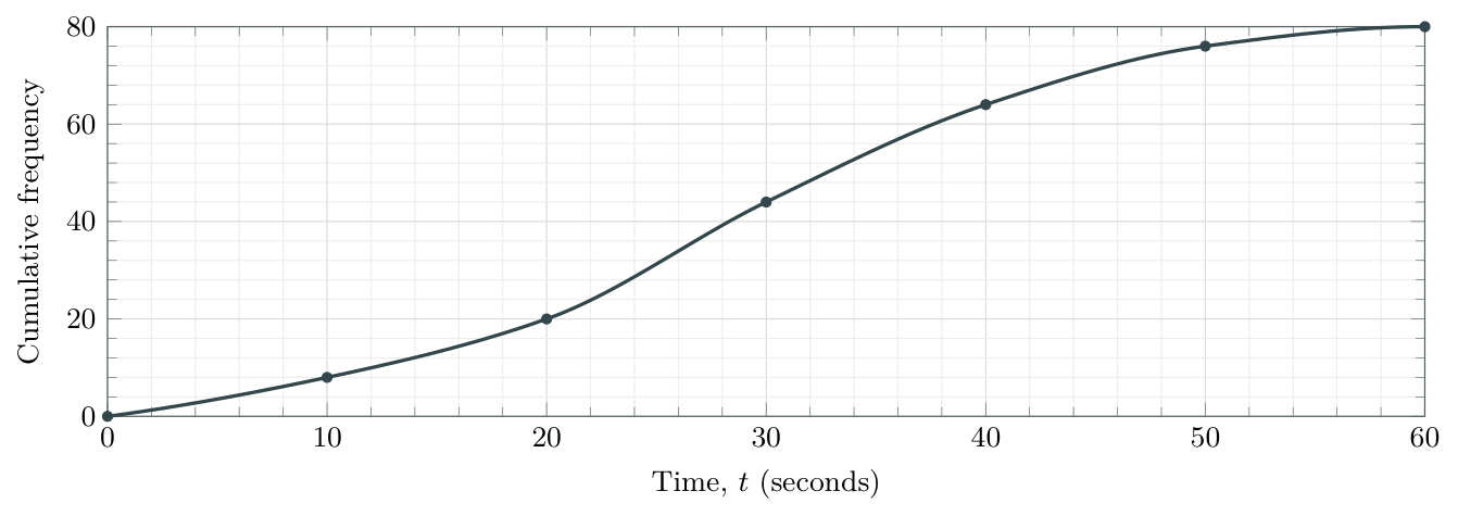
Estimate the percentage who took less than 25 seconds. Hence estimate the probability that a randomly selected participant took less than 25 seconds.
Find the number who took at least 40 seconds.
Find the number whose time satisfies \(20\le t<40\).
Recover the frequency in the class \(30\le t<40\).
Estimate the time exceeded by 10% of participants.
Show the full answer
Solution
(a) Below 25
Go up from 25 seconds and across: \(\text{about }31\) participants. \(\frac{31}{80}\times100\%\approx39\%\). The probability for a randomly selected participant is approximately \(31/80\approx0.39\). Both answers inherit the uncertainty in the graph reading.
(b) At least 40
\(80-64=16\) participants.
(c) Between 20 and 40
\(64-20=44\) participants.
(d) Class frequency
\(64-44=20\) participants (count below 40 minus count below 30).
(e) Upper 10% cutoff
Use \(P_{90}\) at level \(0.9(80)=72\). Read across to the curve, then down: approximately \(46\) seconds.
7. Boundaries and missing detail.
A cumulative-frequency table for masses has boundaries \(100,110,120,130,140\) grams and cumulative frequencies \(0,6,18,30,40\). State the starting point, the sample size and the four ordinary frequencies.
Explain why the exact range is not necessarily \(140-100=40\) grams.
The frequencies for \(0\le x<5\), \(5\le x<10\), \(10\le x<15\), \(15\le x<20\) are \(4,0,9,7\). Find the cumulative frequencies and identify the horizontal part of the graph.
Show the full answer
Solution
(a) Counts
Start \((100,0)\); \(n=40\). Frequencies are \(6,12,12,10\) by subtraction.
(b) Range
The boundaries are not the observed minimum and maximum. The exact range is unknown; 40 g is only a boundary-based approximation.
(c) Empty class
Cumulative frequencies are \(4,4,13,20\) at \(5,10,15,20\). The graph is horizontal at height 4 between \(x=5\) and \(x=10\).
8. Missing box-plot values.
A dataset has minimum 8, \(Q_3=30\), range 34 and IQR 16. Its median is 7 greater than \(Q_1\). There are no outliers.
Determine \(Q_1\), the median and the maximum.
Draw the completed box plot.
State the interval representing the middle half of the data.
Show the full answer
Solution
(a) Recover the three missing measures
\(16=30-Q_1\Rightarrow Q_1=30-16=\boxed{14}\).
Median \(=Q_1+7=14+7=\boxed{21}\), using the stated condition.
\(34=\text{maximum}-8\Rightarrow\text{maximum}=8+34=\boxed{42}\).
(b) Completed plot

(c) Middle half
From 14 to 30. Notice that the median 21 is not the midpoint of these quartiles.
9. Outliers.
The ordered values are 5, 8, 10, 12, 14, 16, 18, 20, 22, 24, 26, 28, 30, 32, 35, 70.
Find the median, \(Q_1\), \(Q_3\) and IQR.
Calculate both fences and identify any outliers.
Draw the modified box plot and state the full range.
Show the full answer
Solution
(a) Summary
Median \(=(20+22)/2=21\); \(Q_1=(12+14)/2=13\); \(Q_3=(28+30)/2=29\). IQR \(=29-13=16\).
(b) Fences
Lower \(=13-1.5(16)=-11\); upper \(=29+1.5(16)=53\). Only 70 is an outlier.
(c) Modified plot and range

Whiskers end at 5 and 35; the full range includes 70: \(70-5=65\).
Independent practice — compare and combine
10. Compare two score distributions.
Both groups took the same test. Group B has one high outlier at 88 and its largest non-outlier is 70. Its other summary values, and Group A’s, are supplied below.
| Group | Minimum | \(Q_1\) | Median | \(Q_3\) | Maximum |
|---|---|---|---|---|---|
| A | 20 | 35 | 47 | 59 | 74 |
| B | 18 | 40 | 49 | 56 | 88 |
Draw both box plots on a common scale.
Compare typical score, middle spread and overall spread, in context.
Which plot gives stronger evidence of symmetry? Explain why this is not proof of normality.
Show the full answer
Solution
(a) Common-scale plots

(b) Comparison
B has a slightly higher median (\(49>47\)), so a typical score is slightly higher. B’s IQR is smaller (\(56-40=16\), compared with \(59-35=24\)), so its middle half is more consistent. But B has the larger range (\(88-18=70\), compared with \(74-20=54\)), partly because of its high outlier.
(c) Symmetry
A has equal box halves (12 each) and equal whiskers (15 each). A gives stronger evidence of symmetry, but a symmetric five-number summary cannot prove a normal, bell-shaped distribution.
11. A fence is a strict threshold.
A dataset has \(Q_1=22\) and \(Q_3=30\).
Find the two outlier fences.
Classify values 9, 10, 42 and 43 as outliers or non-outliers under this rule.
Show the full answer
Solution
(a) Fences
IQR \(=30-22=8\); lower fence \(=22-12=10\); upper fence \(=30+12=42\).
(b) Classification
9 and 43 are outliers; 10 and 42 are not. Equality with a fence is not enough.
12. Diagnose the misunderstanding.
Explain the error in each statement.
“My frequency table has seven different values, so I used \(n=7\), even though the frequencies sum to 45.”
“The cumulative-frequency graph starts at \((0,0)\), so the minimum observation must be zero.”
“Every quarter of a box plot contains exactly 25% of observations strictly between its endpoints, even when values repeat.”
“A symmetric box plot proves that the original distribution is bell-shaped.”
Show the full answer
Solution
(a) Sample size
\(n\) counts observations, so \(n=45\), not the seven distinct labels. Use the frequency list as weights.
(b) Class boundary
The starting point records zero observations below the first lower class boundary; it does not assert an observed value there.
(c) Ties
Quartiles partition positions in ordered data. Repeated values can lie on a cutoff, so strict numerical intervals need not contain exactly 25%.
(d) Shape
Five summary values cannot prove a bell-shaped distribution. Symmetry is only supporting evidence for possible normality.
13. Mixed IB-style extended-response question. [18 marks]
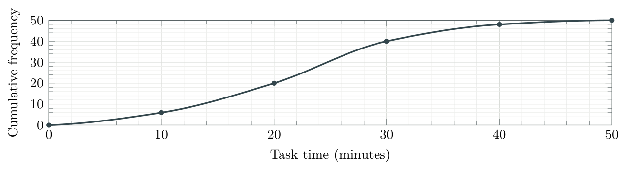
The times \(t\), in minutes, taken by 50 students to complete a project task are grouped below. The actual minimum and maximum are 2 and 47 minutes; no outliers were identified.
| \(t\) (min) | \(0\le t<10\) | \(10\le t<20\) | \(20\le t<30\) | \(30\le t<40\) | \(40\le t<50\) |
|---|---|---|---|---|---|
| Frequency | 6 | 14 | 20 | 8 | 2 |
Construct a cumulative-frequency table.[2]
Draw a cumulative-frequency graph using a smooth curve through the points.[3]
Estimate the median and IQR.[4]
Estimate the time above which the slowest 10% of students lie.[2]
Estimate the number whose time satisfies \(15\le t<35\).[3]
Find the range.[1]
Draw a box plot using the known extremes and estimated quartiles.[3]
Show the full answer
Solution
(a) Table
Boundaries \(0,10,20,30,40,50\) have cumulative frequencies \(0,6,20,40,48,50\).
(b) Graph
(c) Median and IQR
Read across at levels \(12.5,25,37.5\), then down to time. To the nearest minute on the displayed curve, \[Q_1\approx15,\qquad \text{median}\approx23,\qquad Q_3\approx28.\] Hence IQR \(\approx28-15=\boxed{13\text{ minutes}}\).
(d) Slowest 10%
Use level \(0.90(50)=45\): read \(\boxed{P_{90}\approx35\text{ minutes}}\).
(e) Between 15 and 35
Read about 12 participants below 15 minutes and about 45 below 35 minutes. The estimate is \(45-12=\boxed{33\text{ students}}\).
(f) Range
\(47-2=\boxed{45\text{ minutes}}\), using the actual extremes.
(g) Box plot
Use the same rounded quartiles as in part (c), with the known extremes 2 and 47.

AI SL consolidation — technology and interpretation
Use your graphical calculator when helpful. Show the key numerical results and explain what they mean in the context of each question.
14. Calls to a help desk [7 marks]
The number of calls received in each of 40 one-hour periods is recorded below.
| Calls, \(x\) | 0 | 1 | 2 | 3 | 4 | 5 |
|---|---|---|---|---|---|---|
| Frequency, \(f\) | 4 | 8 | 12 | 8 | 6 | 2 |
Verify that the table represents 40 one-hour periods.[1]
Use technology to find \(Q_1\), the median and \(Q_3\) for the number of calls.[3]
One recorded period is selected at random, each equally likely. Find the probability that at least four calls were received.[2]
Interpret the median in this context.[1]
Show the full answer
Solution
(a) Total
\(4+8+12+8+6+2=40\) one-hour periods.
(b) Calculator summaries
Enter \(0,1,2,3,4,5\) as the data list and \(4,8,12,8,6,2\) as its frequency list. One-Variable Statistics gives \(\boxed{Q_1=1,\ \text{median}=2,\ Q_3=3}\) calls. Check \(n=40\), not 6.
(c) Probability
At least four means 4 or 5 calls: \(\dfrac{6+2}{40}=\dfrac8{40}=\boxed{0.20}\).
(d) Interpretation
The median is 2 calls per one-hour period: it describes the central recorded number, not a frequency of periods. Repeated values mean the median does not imply exactly half of the periods had strictly fewer than 2 calls.
15. Comparing delivery times [7 marks]
Two delivery services record their delivery times, in minutes. Their summaries are shown below. For service B, the greatest non-outlier time is 30 minutes.
| Service | Minimum | \(Q_1\) | Median | \(Q_3\) | Maximum |
|---|---|---|---|---|---|
| A | 6 | 12 | 18 | 24 | 32 |
| B | 5 | 14 | 17 | 22 | 45 |
Calculate the IQR for each service.[2]
Show that the 45-minute delivery for service B is an outlier.[2]
A customer prefers a lower typical delivery time and a more consistent middle half. Which service better meets both preferences? Justify your answer.[2]
State the upper-whisker endpoint for service B’s modified box plot.[1]
Show the full answer
Solution
(a) Spread
Service A: \(24-12=\boxed{12\text{ minutes}}\). Service B: \(22-14=\boxed{8\text{ minutes}}\).
(b) Outlier
For B, the upper fence is \(22+1.5(8)=34\) minutes. Since \(45>34\), the 45-minute delivery is an outlier.
(c) Comparison
Service B: its median is lower (\(17<18\) minutes) and its IQR is smaller (\(8<12\) minutes). It has a lower typical delivery time and less spread in the middle half, but it does not have the smaller full range.
(d) Whisker
\(\boxed{30\text{ minutes}}\), the stated greatest non-outlier. Neither the fence 34 nor the outlier 45 is the endpoint.
Ready to work independently?
You should be able to explain why cumulative points use upper boundaries, read counts and percentiles in both directions, distinguish exact values from grouped estimates, build an outlier-aware box plot and justify comparisons in context.
A correct answer obtained only by matching a worked example is not yet reliable mastery. Revisit the section for any question where you could not choose and explain the method yourself.
Tutorial reference list
| Types of data | https://youtu.be/AxWhr60hRuw |
|---|---|
| Cumulative-frequency diagrams | https://youtu.be/fUjKmcjn6w4 |
| TI-Nspire: statistics from a raw list | https://youtu.be/x_LLRlNLjxk |
| TI-Nspire: frequency-table statistics | https://youtu.be/SIDvdYm_A3E |
Answer key and solution outlines
Graphical estimates must be consistent with the displayed curve and its scale. The answers below use rounded readings from the shown curves; slightly different reasonable readings may follow from another carefully drawn curve. Do not report unjustified decimal places.
1. Data and boundaries
Solution
(a) Types
Late-arrival count: discrete. Parcel mass and running time: continuous.
(b) Boundary
\(t=20\) belongs to \(20\le t<30\); width \(=30-20=10\).
(c) Suitable graph
A histogram displays the grouped distribution of running times on a numerical scale. A cumulative-frequency graph is also suitable when the aim is to read percentages or percentile times.
2. Discrete frequency distribution
Solution
(a) Table
| Puzzles | 0 | 1 | 2 | 3 | 4 | Total |
|---|---|---|---|---|---|---|
| Frequency | 1 | 2 | 3 | 2 | 4 | 12 |
(b) Mode
4 puzzles: this value has the greatest frequency, 4.
(c) Percentage
At least three puzzles: \(2+4=6\) students. \(\frac6{12}\times100\%=50\%\).
3. Raw-data quartiles
Solution
(a) Order
\(4,6,7,10,11,13,15,19\).
(b) Centre and quartiles
Median \(=(10+11)/2=10.5\); \(Q_1=(6+7)/2=6.5\); \(Q_3=(13+15)/2=14\).
(c) Spread
Range \(=19-4=15\); IQR \(=14-6.5=7.5\).
4. Clinic histogram
Solution
(a) Histogram and modal class
The modal class is \(20\le t<30\) minutes. All six rectangles occupy intervals of width 10.
(b) Number
\(7+12+9=28\) patients have \(10\le t<40\).
(c) Percentage
There are \(n=40\) patients; \(3+7+12=22\) have \(t<30\). \(\frac{22}{40}\times100\%=55\%\).
Answers — cumulative-frequency methods
5. Clinic cumulative frequency
Solution
(a) Table and graph
| Waiting time below (min) | 0 | 10 | 20 | 30 | 40 | 50 | 60 |
|---|---|---|---|---|---|---|---|
| Cumulative frequency | 0 | 3 | 10 | 22 | 31 | 37 | 40 |
(b) Quartiles and IQR
With \(n=40\), read at levels 10, 20 and 30. To the nearest minute, \[Q_1\approx20,\qquad\text{median}\approx28,\qquad Q_3\approx39\text{ minutes}.\] \[\operatorname{IQR}\approx39-20=19\text{ minutes}.\]
(c) 90th percentile
Use \(0.9(40)=36\). Read across to the curve and down: \(P_{90}\approx48\) minutes. Approximately 90% waited no longer than this; about 10% waited longer.
6. Completion times
Solution
(a) Below 25
Go up from 25 seconds and across: \(\text{about }31\) participants. \(\frac{31}{80}\times100\%\approx39\%\). The probability for a randomly selected participant is approximately \(31/80\approx0.39\). Both answers inherit the uncertainty in the graph reading.
(b) At least 40
\(80-64=16\) participants.
(c) Between 20 and 40
\(64-20=44\) participants.
(d) Class frequency
\(64-44=20\) participants (count below 40 minus count below 30).
(e) Upper 10% cutoff
Use \(P_{90}\) at level \(0.9(80)=72\). Read across to the curve, then down: approximately \(46\) seconds.
7. Boundaries and missing detail
Solution
(a) Counts
Start \((100,0)\); \(n=40\). Frequencies are \(6,12,12,10\) by subtraction.
(b) Range
The boundaries are not the observed minimum and maximum. The exact range is unknown; 40 g is only a boundary-based approximation.
(c) Empty class
Cumulative frequencies are \(4,4,13,20\) at \(5,10,15,20\). The graph is horizontal at height 4 between \(x=5\) and \(x=10\).
Answers — box plots and comparisons
8. Missing box-plot values
Solution
(a) Recover the three missing measures
\(16=30-Q_1\Rightarrow Q_1=30-16=\boxed{14}\).
Median \(=Q_1+7=14+7=\boxed{21}\), using the stated condition.
\(34=\text{maximum}-8\Rightarrow\text{maximum}=8+34=\boxed{42}\).
(b) Completed plot
(c) Middle half
From 14 to 30. Notice that the median 21 is not the midpoint of these quartiles.
9. Outliers
Solution
(a) Summary
Median \(=(20+22)/2=21\); \(Q_1=(12+14)/2=13\); \(Q_3=(28+30)/2=29\). IQR \(=29-13=16\).
(b) Fences
Lower \(=13-1.5(16)=-11\); upper \(=29+1.5(16)=53\). Only 70 is an outlier.
(c) Modified plot and range
Whiskers end at 5 and 35; the full range includes 70: \(70-5=65\).
10. Compare the score distributions
Solution
(a) Common-scale plots
(b) Comparison
B has a slightly higher median (\(49>47\)), so a typical score is slightly higher. B’s IQR is smaller (\(56-40=16\), compared with \(59-35=24\)), so its middle half is more consistent. But B has the larger range (\(88-18=70\), compared with \(74-20=54\)), partly because of its high outlier.
(c) Symmetry
A has equal box halves (12 each) and equal whiskers (15 each). A gives stronger evidence of symmetry, but a symmetric five-number summary cannot prove a normal, bell-shaped distribution.
11. Strict outlier thresholds
Solution
(a) Fences
IQR \(=30-22=8\); lower fence \(=22-12=10\); upper fence \(=30+12=42\).
(b) Classification
9 and 43 are outliers; 10 and 42 are not. Equality with a fence is not enough.
Answers — misconceptions and the mixed question
12. Diagnose the error
Solution
(a) Sample size
\(n\) counts observations, so \(n=45\), not the seven distinct labels. Use the frequency list as weights.
(b) Class boundary
The starting point records zero observations below the first lower class boundary; it does not assert an observed value there.
(c) Ties
Quartiles partition positions in ordered data. Repeated values can lie on a cutoff, so strict numerical intervals need not contain exactly 25%.
(d) Shape
Five summary values cannot prove a bell-shaped distribution. Symmetry is only supporting evidence for possible normality.
13. Mixed IB-style question
Solution
(a) Table
Boundaries \(0,10,20,30,40,50\) have cumulative frequencies \(0,6,20,40,48,50\).
(b) Graph
(c) Median and IQR
Read across at levels \(12.5,25,37.5\), then down to time. To the nearest minute on the displayed curve, \[Q_1\approx15,\qquad \text{median}\approx23,\qquad Q_3\approx28.\] Hence IQR \(\approx28-15=\boxed{13\text{ minutes}}\).
(d) Slowest 10%
Use level \(0.90(50)=45\): read \(\boxed{P_{90}\approx35\text{ minutes}}\).
(e) Between 15 and 35
Read about 12 participants below 15 minutes and about 45 below 35 minutes. The estimate is \(45-12=\boxed{33\text{ students}}\).
(f) Range
\(47-2=\boxed{45\text{ minutes}}\), using the actual extremes.
(g) Box plot
Use the same rounded quartiles as in part (c), with the known extremes 2 and 47.
Answers — AI SL consolidation and checkpoints
14. Calls to a help desk
Solution
(a) Total
\(4+8+12+8+6+2=40\) one-hour periods.
(b) Calculator summaries
Enter \(0,1,2,3,4,5\) as the data list and \(4,8,12,8,6,2\) as its frequency list. One-Variable Statistics gives \(\boxed{Q_1=1,\ \text{median}=2,\ Q_3=3}\) calls. Check \(n=40\), not 6.
(c) Probability
At least four means 4 or 5 calls: \(\dfrac{6+2}{40}=\dfrac8{40}=\boxed{0.20}\).
(d) Interpretation
The median is 2 calls per one-hour period: it describes the central recorded number, not a frequency of periods. Repeated values mean the median does not imply exactly half of the periods had strictly fewer than 2 calls.
15. Comparing delivery times
Solution
(a) Spread
Service A: \(24-12=\boxed{12\text{ minutes}}\). Service B: \(22-14=\boxed{8\text{ minutes}}\).
(b) Outlier
For B, the upper fence is \(22+1.5(8)=34\) minutes. Since \(45>34\), the 45-minute delivery is an outlier.
(c) Comparison
Service B: its median is lower (\(17<18\) minutes) and its IQR is smaller (\(8<12\) minutes). It has a lower typical delivery time and less spread in the middle half, but it does not have the smaller full range.
(d) Whisker
\(\boxed{30\text{ minutes}}\), the stated greatest non-outlier. Neither the fence 34 nor the outlier 45 is the endpoint.
Checkpoint answers — use these to diagnose a gap
| 1 | Values \(0,1,2\) have frequencies \(1,2,3\). \(n=6\); mode 2; percentage equal to 2 is \(3/6\times100\%=50\%\). |
| 2 | (a) Position \(4.5\); median \(=10\); \(Q_1=6\); \(Q_3=14\); range \(=14\); IQR \(=8\).(b) Position \(5\); median \(=11\); exclude it from both halves. \(Q_1=6\); \(Q_3=16\); range \(=16\); IQR \(=10\). |
| 3 | Width 10; 20 is excluded. The three frequencies are \(1,2,1\). An empty class keeps its interval on the scale but has no visible bar. |
| 4 | Levels \(30,60,90,114\). They are counts on the vertical axis, not the percentile values; read across and down. |
| 5 | Below 12: \(28/80\times100\%=35\%\). At least 18: \(80-46=34\). From 12 to below 18: \(46-28=18\). |
| 6 | Range \(=40-5=35\); IQR \(=25-12=13\); middle-half interval from 12 to 25. |
| 7 | IQR \(=8\); fences \(-2\) and \(30\). 30 is not an outlier; 31 is. |
| 8 | No: symmetry does not establish normality. Neither mean nor sample size is generally recoverable from an unannotated box plot. |
Source scope. Syllabus checked against the supplied Mathematics: applications and interpretation guide, SL 4.2 (printed page 52; first assessment 2021), with supporting links to SL 4.1 and 4.3. Original questions use AI SL-style command terms, calculator use and contextual interpretation; this is not an official IB publication.
Keep the distinction clear: a frequency is a count; a quartile is a value of the variable; a graphical reading from grouped data is an estimate.
Back to lesson overview ↑