IB Mathematics: Applications and Interpretation SL — Topic 5 Calculus

Trapezoidal Rule for Integration

Approximate areas and definite integrals from a table of data or a function using equal-width intervals.

AI SL · SL 5.8

Learning goal

Approximate an area or definite integral from a table of data or a function, using equal-width intervals and the trapezoidal rule.

Syllabus link

IB Mathematics AI SL: SL 5.8. Approximate areas using the trapezoidal rule from a table of data or a function, with intervals of equal width.

Big idea

Approximate the area under the curve as the sum of the areas of trapezia (trapeziums). The more trapezia we use, the more accurate the estimate becomes.

Key relationship

For n equal intervals, \(h=\frac{b-a}{n}\), with the two endpoint ordinates used once and every middle ordinate used twice.

Why do we need an approximation?

A definite integral such as

\[ \int_a^b f(x)\,dx \]

represents an accumulated quantity. When the graph lies above the horizontal axis, it can represent the area under a curve. However, we may not know an antiderivative, or the information may be available only as measured data in a table.

The trapezoidal rule gives a practical approximation by joining consecutive points with straight-line segments.

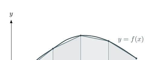
A smooth curve with four equal-width trapezia underneath it, illustrating a trapezoidal approximation — The curved boundary is replaced by straight-line chords. The shaded trapezia approximate the region under the curve.

Notice. The shaded region is an approximation of the area enclosed by the curve and the x-axis. This approximation is equal to the sum of the areas of the trapezia.

Key idea. Approximate the area under the curve as the sum of the areas of the trapezia. The more trapezia we use, the more accurate the estimate becomes.

From one trapezium to the general formula

For one interval of width \(h\), with vertical heights \(y_0\) and \(y_1\), the area of the trapezium is

\[ A_1=\frac12 h(y_0+y_1). \]

One trapezium with area one half h times y zero plus y one, beside four trapezia with five vertical ordinates — Four trapezia require five vertical heights: \(y_0,y_1,y_2,y_3,y_4\).

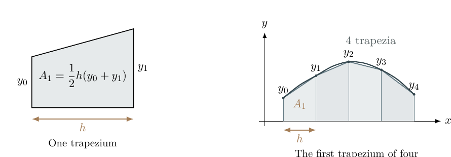
Notice. The single trapezium on the left is the first trapezium, \(A_1\). If a region is divided into 4 trapezia, there are \(4+1=5\) vertical heights.

If the interval \([a,b]\) is divided into \(n\) equal parts, then

\[ h=\frac{b-a}{n}. \]

There are \(n\) trapezia but \(n+1\) vertical heights, labelled \(y_0,y_1,\ldots,y_n\).

Adding all the trapezia gives

\[ \begin{aligned} \int_a^b y\,dx &\approx \frac12h(y_0+y_1)+\frac12h(y_1+y_2)+\cdots+\frac12h(y_{n-1}+y_n)\\[2mm] &=\frac12h\Big[(y_0+y_1)+(y_1+y_2)+\cdots+(y_{n-1}+y_n)\Big]\\[2mm] &=\frac12h\Big[y_0+y_1+y_1+y_2+\cdots+y_{n-1}+y_{n-1}+y_n\Big]\\[2mm] &=\frac12h\Big[y_0+2y_1+2y_2+\cdots+2y_{n-1}+y_n\Big]\\[2mm] &=\frac12h\Big[(y_0+y_n)+2(y_1+y_2+\cdots+y_{n-1})\Big]. \end{aligned} \]

\[ \boxed{\int_a^b y\,dx\approx \frac12h\Big[(y_0+y_n)+2(y_1+y_2+\cdots+y_{n-1})\Big]}, \qquad h=\frac{b-a}{n} \]

\(n\): number of equal intervals, and therefore the number of trapezia
\(h\): width of each interval
\(y_0\) and \(y_n\): first and last ordinates; each is used once
\(y_1,\ldots,y_{n-1}\): middle ordinates; each is used twice

Worked example 1: a function and a given number of intervals

Worked example 1: estimate an integral using \(n=4\)

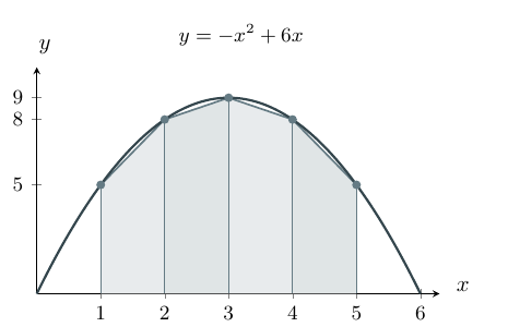
Use the trapezoidal rule with four equal intervals to estimate

\[ \int_1^5(-x^2+6x)\,dx. \]

Step 1: find the interval width.

Recall that \(h=\frac{b-a}{n}\).

Here:

\(a=1\) and \(b=5\) are the lower and upper limits of the integral;
\(n=4\) comes from the instruction to use four equal intervals.

\[ h=\frac{b-a}{n}=\frac{5-1}{4}=1. \]

Step 2: build the table of values.

\(x\)	1	2	3	4	5
\(y=-x^2+6x\)	5	8	9	8	5

Step 3: substitute into the formula.

\[ \begin{aligned} \int_1^5(-x^2+6x)\,dx &\approx \frac12(1)\Big[(5+5)+2(8+9+8)\Big]\\ &=\frac12(10+50)\\ &=30. \end{aligned} \]

Estimate: \(\displaystyle \int_1^5(-x^2+6x)\,dx\approx30\) square units.

Using a GDC to evaluate the integral gives the actual value

\[ \frac{92}{3}\approx30.7. \]

The trapezoidal estimate is slightly smaller because this curve is concave down on the interval: the straight chords lie below the curve.

Graph of y equals negative x squared plus six x with four trapezia between x equals one and x equals five — The chords lie below this concave-down parabola, giving an underestimate.

When the interval width \(h\) is given

Sometimes the question gives \(h\) rather than \(n\). In that case,

\[ n=\frac{b-a}{h}. \]

Start at \(x=a\) and repeatedly add \(h\) until reaching \(x=b\).

The full table must begin at \(a\), finish at \(b\), and contain \(n+1\) ordinates.

Worked example 2: build a table from a function

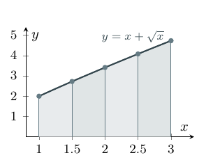
Use the trapezoidal rule with \(h=0.5\) to estimate

\[ \int_1^3\left(x+\sqrt{x}\right)\,dx. \]

Step 1: determine the number of intervals.

We start with the formula for the interval width:

\[ h=\frac{b-a}{n}. \]

Multiply both sides by \(n\):

\[ nh=b-a. \]

Then divide both sides by \(h\):

\[ n=\frac{b-a}{h}. \]

The lower and upper limits give \(a=1\) and \(b=3\), while the question gives \(h=0.5\). Therefore

\[ n=\frac{b-a}{h}=\frac{3-1}{0.5}=4. \]

Hence there are 4 equal intervals and \(4+1=5\) x-values.

Step 2: calculate the ordinates.

\(x\)	1	1.5	2	2.5	3
\(y=x+\sqrt{x}\)	2.0000	2.7247	3.4142	4.0811	4.7321

Step 3: apply the trapezoidal rule.

\[ \begin{aligned} \int_1^3(x+\sqrt{x})\,dx &\approx \frac12(0.5)\Big[(2.0000+4.7321)\\ &\qquad\qquad +2(2.7247+3.4142+4.0811)\Big]\\ &\approx 6.7931. \end{aligned} \]

Estimate: \(\displaystyle \int_1^3(x+\sqrt{x})\,dx\approx6.79\) square units.

Graph of y equals x plus square root x with trapezia of width 0.5 from x equals one to x equals three — Five ordinates create four equal-width trapezia.

Using measured data

The formula is especially useful when the boundary is irregular and is known only from measurements. If \(y\) is the perpendicular distance from a straight baseline to a boundary, then

\[ \int_a^b y\,dx \]

represents the area between the baseline and the boundary.

The same method also applies to accumulated quantities such as energy, total flow, displacement or total production. In those settings, the units are the product of the axis units rather than “square units”.

Horizontal variable	Vertical variable	Units of the integral
metres	metres	\(\mathrm{m}^2\)
hours	kilowatts	kilowatt-hours (kWh)
minutes	litres per minute	litres
seconds	metres per second	metres

Worked example 3: measurements, a model and percentage error

Worked example 3: estimate the area of a wetland

A straight path runs alongside a small wetland. The perpendicular distance \(y\) metres from the path to the edge of the wetland is measured every 3 metres.

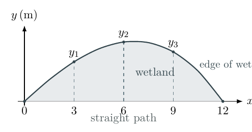
Wetland boundary measured at x equals zero, three, six, nine and twelve metres from a straight path — The irregular boundary is sampled at equal 3 m intervals along the straight path.

\(x\) (m)	0	3	6	9	12
\(y\) (m)	0	2.4	3.6	3.0	0

(a) Estimate the area using the trapezoidal rule.

Here \(h=3\) and there are four equal intervals.

\[ \begin{aligned} A_{\mathrm T} &\approx \frac12(3)\Big[(0+0)+2(2.4+3.6+3.0)\Big]\\ &=27. \end{aligned} \]

Trapezoidal estimate: \(A_{\mathrm T}\approx27\ \mathrm{m}^2\).

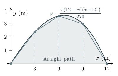
Wetland model curve and straight-line trapezoidal chords through the measured points — The smooth model can be compared with the trapezoidal chords through the measured points.

(b) A model for the edge is \(y=\dfrac{x(12-x)(x+21)}{270}\), for \(0\leq x\leq12\). Write an integral for the modelled area and use a GDC to calculate it.

\[ A=\int_0^{12}\frac{x(12-x)(x+21)}{270}\,dx=28.8\ \mathrm{m}^2. \]

\[ \begin{aligned} \text{percentage error} &=\left|\frac{\text{estimate}-\text{actual}}{\text{actual}}\right|\times100\%\\ &=\left|\frac{27-28.8}{28.8}\right|\times100\%\\ &=6.25\%. \end{aligned} \]

Percentage error: \(6.25\%\).

Accuracy: overestimates, underestimates and interval width

The trapezoidal rule replaces each part of the curve by a chord.

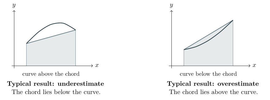
Concave-down curve where the trapezoidal chord lies below the curve and concave-up curve where the chord lies above the curve — For a concave-down curve, the chord typically lies below the curve; for a concave-up curve, it typically lies above.

Concave down: typical underestimate. The chord lies below the curve.

Concave up: typical overestimate. The chord lies above the curve.

What improves the approximation? Using more intervals makes \(h\) smaller. The line segments then follow the curve more closely, so the approximation usually improves. If the graph changes concavity, do not rely only on a visual overestimate/underestimate rule; calculate the estimate and compare when an actual value is available.

A reliable AI SL method

Identify the information. Record \(a\), \(b\), and either \(n\) or \(h\).
Check equal spacing. The compact AI SL formula assumes equal-width intervals.
Calculate the missing quantity. Use \(h=(b-a)/n\) or \(n=(b-a)/h\).
Create the complete table. There must be \(n+1\) ordinates.
Separate endpoints and middle values. The endpoints are used once; every middle ordinate is doubled.
Calculate before rounding. Keep several decimal places in the table and round only the final answer unless instructed otherwise.
State units and meaning. Interpret the estimated accumulated quantity in context.

Common mistakes

Mistake	Correction
Using \(n\) as the number of ordinates	\(n\) is the number of intervals; there are \(n+1\) ordinates.
Doubling \(y_0\) and \(y_n\)	Only the middle ordinates are multiplied by 2.
Using \(h=b-a\)	Divide by the number of intervals: \(h=(b-a)/n\).
Applying the compact formula to unequal gaps	First check that consecutive x-values differ by the same amount.
Rounding every table entry too early	Store full GDC values and round the final estimate.
Writing “square units” in every context	Multiply the horizontal and vertical units; for example kW × h gives kWh.

Vocabulary note. An ordinate is another term for a y-value. So, for example, “\(n+1\) ordinates” means “\(n+1\) y-values.”

Practice

Practice 1: direct use of a table

Use the trapezoidal rule to estimate \(\displaystyle\int_0^4 f(x)\,dx\) from the table.

\(x\)	0	1	2	3	4
\(f(x)\)	2.0	3.1	4.6	6.4	8.5

Practice 2: generate values from a function

Use four equal intervals to estimate

\[ \int_0^4\bigl(2+\ln(x+1)\bigr)\,dx. \]

Give your answer to three decimal places.

Practice 3: count intervals and ordinates

The interval \([1,2]\) is divided using \(h=0.25\).

Find \(n\).
List all the x-values needed for the trapezoidal rule.
State the number of ordinates.

Practice 4: solar-energy context

The power output \(P\) kW of a solar installation is measured over six hours.

\(t\) (h)	0	1	2	3	4	5	6
\(P\) (kW)	0	0.8	2.1	3.0	2.4	1.1	0

Estimate the electrical energy generated. Give the correct unit.

Practice 5: irregular boundary

A surveyor measures the perpendicular distance from a straight baseline to the edge of a reservoir.

\(x\) (m)	0	5	10	15	20
\(y\) (m)	0	6.2	8.1	5.6	0

Estimate the area between the baseline and the edge of the reservoir.

Practice 6: estimate, actual value and percentage error

For \(f(x)=x^2+1\) on \(0\leq x\leq2\):

Use four equal intervals to estimate \(\displaystyle\int_0^2 f(x)\,dx\).
Use a GDC or an antiderivative to find the actual value.
Find the percentage error in the trapezoidal estimate.
Explain whether the estimate is an overestimate or an underestimate.

Practice 7: a missing ordinate

The trapezoidal rule with \(h=2\) is used with the ordinates

\[ y_0=1.2,\quad y_1=2.0,\quad y_2=k,\quad y_3=3.1,\quad y_4=3.4. \]

The resulting estimate is 20.8. Find \(k\).

Practice 8: mixed IB-style application

The cross-section of a landscaped garden is bounded by a straight path and a smooth curve. The perpendicular heights are measured at equal intervals.

\(x\) (m)	0	2	4	6	8
\(y\) (m)	0	1.8	2.5	1.7	0

Use the trapezoidal rule to estimate the cross-sectional area. [2]
A model for the curve is \(y=0.16x(8-x)\), \(0\leq x\leq8\). Write down an integral for the modelled area. [1]
Calculate the modelled area. [1]
Find the percentage error in the trapezoidal estimate. [2]

Answer key

Practice 1

Here \(h=1\).

\[ \begin{aligned} \int_0^4f(x)\,dx &\approx \frac12(1)\Big[(2.0+8.5)+2(3.1+4.6+6.4)\Big]\\ &=19.35. \end{aligned} \]

Answer: 19.35 square units.

Practice 2

The x-values are \(0,1,2,3,4\), and

\(x\)	0	1	2	3	4
\(2+\ln(x+1)\)	2.0000	2.6931	3.0986	3.3863	3.6094

\[ \begin{aligned} \int_0^4(2+\ln(x+1))\,dx &\approx \frac12\Big[(2.0000+3.6094)\\ &\qquad +2(2.6931+3.0986+3.3863)\Big]\\ &\approx11.983. \end{aligned} \]

Practice 3

\[n=\frac{2-1}{0.25}=4.\]

The five x-values are \(1,\ 1.25,\ 1.50,\ 1.75,\ 2\). There are \(n+1=5\) ordinates.

Practice 4

Here \(h=1\) hour.

\[ \begin{aligned} E&\approx\frac12(1)\Big[(0+0)+2(0.8+2.1+3.0+2.4+1.1)\Big]\\ &=9.4. \end{aligned} \]

Answer: approximately \(9.4\ \mathrm{kWh}\).

Practice 5

Here \(h=5\) metres.

\[ \begin{aligned} A&\approx\frac12(5)\Big[(0+0)+2(6.2+8.1+5.6)\Big]\\ &=99.5. \end{aligned} \]

Answer: approximately \(99.5\ \mathrm{m}^2\).

Practice 6

With \(h=0.5\), the ordinates are \(1,\ 1.25,\ 2,\ 3.25,\ 5\).

\[ A_{\mathrm T}\approx\frac12(0.5)\Big[(1+5)+2(1.25+2+3.25)\Big]=4.75. \]

The actual value is

\[ \int_0^2(x^2+1)\,dx=\frac{14}{3}\approx4.6667. \]

Hence

\[ \text{percentage error}=\left|\frac{4.75-14/3}{14/3}\right|\times100\%\approx1.79\%. \]

Because \(x^2+1\) is concave up, the chords lie above the curve and the trapezoidal rule gives an overestimate.

Practice 7

\[ \begin{aligned} 20.8 &=\frac12(2)\Big[(1.2+3.4)+2(2.0+k+3.1)\Big]\\ &=14.8+2k. \end{aligned} \]

Therefore \(2k=6\), so \(\boxed{k=3}\).

Practice 8

(a) Here \(h=2\):

\[ A_{\mathrm T}\approx\frac12(2)\Big[(0+0)+2(1.8+2.5+1.7)\Big]=12\ \mathrm{m}^2. \]

(b)

\[ A=\int_0^8 0.16x(8-x)\,dx. \]

(c) Using a GDC, \(A\approx13.6533\ \mathrm{m}^2\).

(d)

\[ \text{percentage error}=\left|\frac{12-13.6533}{13.6533}\right|\times100\%\approx12.1\%. \]

Contact / enquiry

Trapezoidal Rule for Integration

Learning goal

Syllabus link

Big idea

Key relationship

Why do we need an approximation?

From one trapezium to the general formula

Worked example 1: a function and a given number of intervals

Worked example 1: estimate an integral using \(n=4\)

Related tutorial 1: Understanding and deriving the trapezoidal rule

When the interval width \(h\) is given

Worked example 2: build a table from a function

Related tutorial 2: Using the trapezoidal rule when \(h\) is given

Using measured data

Worked example 3: measurements, a model and percentage error

Worked example 3: estimate the area of a wetland

Related tutorial 3: An IB-style context - data, model and percentage error

Accuracy: overestimates, underestimates and interval width

A reliable AI SL method

Practice

Practice 1: direct use of a table

Practice 2: generate values from a function

Practice 3: count intervals and ordinates

Practice 4: solar-energy context

Practice 5: irregular boundary

Practice 6: estimate, actual value and percentage error

Practice 7: a missing ordinate

Practice 8: mixed IB-style application

Answer key

Practice 1

Practice 2

Practice 3

Practice 4

Practice 5

Practice 6

Practice 7

Practice 8

Related Radford Mathematics tutorials