IB Mathematics: Analysis and Approaches SL/HL — Topic 5 Calculus

Limits and the Derivative

Approach a value numerically and graphically, then use the same limiting idea to understand instantaneous gradient and rate of change.

AA SL/HL · SL 5.1

Learning goal

Estimate limits from tables and graphs, then interpret a derivative both as the gradient of a curve and as an instantaneous rate of change.

Syllabus link

IB Mathematics AA SL/HL: SL 5.1. Informal understanding of limits and the derivative; formal analytic methods for evaluating limits are not required.

Big idea

A limit describes what a function is approaching. A derivative describes what a gradient or quantity is doing at an instant.

Key relationship

$f'(a)=\displaystyle\lim_{h\to0}\frac{f(a+h)-f(a)}{h}$ connects secant gradients with the tangent gradient.

Approaching a value: the idea of a limit

A limit is about nearby behaviour. We ask what value the output is approaching as the input gets closer and closer to a chosen number.

Limit notation

\[\lim_{x\to a}f(x)=L\]

This reads: “as $x$ approaches $a$, $f(x)$ approaches $L$.” The value of $f(a)$ itself may be different from $L$, or $f(a)$ may not even be defined.

At AA SL/HL, the emphasis is on understanding limits from tables, graphs and the idea of approaching a value. We are not trying to build a formal algebraic theory of limits.

Estimating a limit from a table and from a graph

Worked example 1: estimating a limit numerically

Estimate

\[\lim_{x\to2}\frac{x^2-4}{x-2}.\]

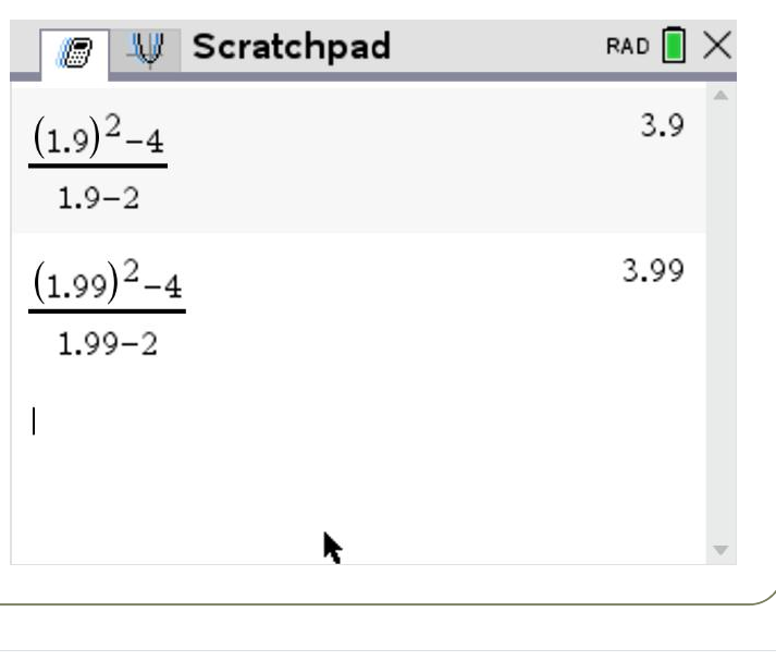
Substituting $x=2$ gives $\frac00$, so instead we look at values of $x$ very close to 2 from both sides.

$x$	1.9	1.99	1.999	2.001	2.01	2.1
$\frac{x^2-4}{x-2}$	3.9	3.99	3.999	4.001	4.01	4.1

The values approach 4 from both sides, so

\[\boxed{\lim_{x\to2}\frac{x^2-4}{x-2}=4}.\]

Calculator table showing values of the expression approaching 4 as x approaches 2 — The numerical table in the handout makes the “approach from both sides” idea visible.

A limit need not equal the function value

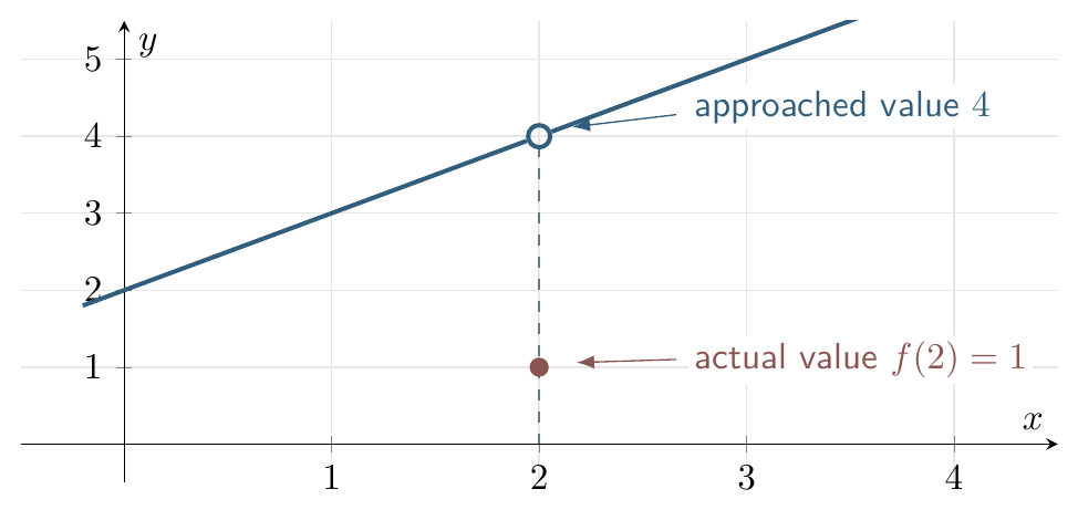
Suppose the graph approaches $y=4$ as $x\to2$, but the filled point at $x=2$ is at $y=1$. Then

\[\lim_{x\to2}f(x)=4\qquad\text{but}\qquad f(2)=1.\]

The limit describes what nearby outputs approach; the function value describes the actual output at the point.

Graph with an open circle at y equals 4 and a filled point at y equals 1 when x equals 2 — The open circle shows the approached value; the filled point shows the actual function value.

When a two-sided limit does not exist

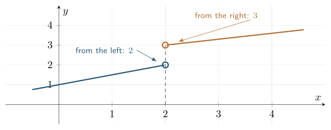
A two-sided limit exists only when the function approaches the same value from the left and from the right.

Different one-sided behaviour

If the left-hand values approach 2 while the right-hand values approach 3, there is no single number that the function approaches from both sides. Therefore the two-sided limit does not exist.

\[\lim_{x\to a^-}f(x)=2,\qquad \lim_{x\to a^+}f(x)=3\quad\Longrightarrow\quad \lim_{x\to a}f(x)\text{ does not exist}.\]

Graph showing different left-hand and right-hand limiting values — For a two-sided limit, approaching from both directions must lead to the same value.

From straight-line gradient to the gradient of a curve

The derivative answers a new question: how steep is a curve at one particular point?

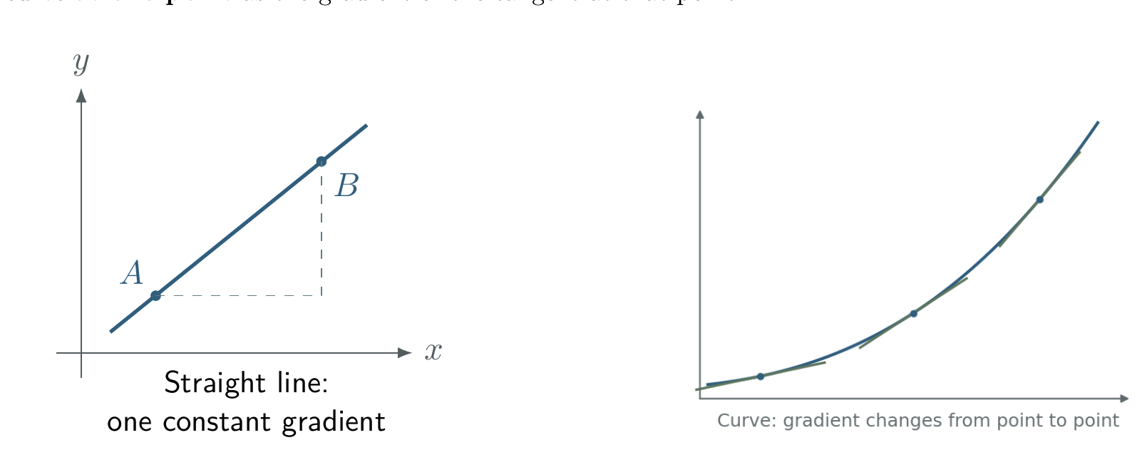
For a straight line, the gradient is constant:

\[m=\frac{\Delta y}{\Delta x}.\]

For a curve, the gradient changes from point to point. At one point we measure the gradient of the tangent to the curve.

Derivative at a point

$f'(a)$ is the gradient of the tangent to $y=f(x)$ at $x=a$.

Comparison of a constant straight-line gradient with a tangent gradient on a curve — A straight line has one gradient; a curve has a different tangent gradient at different points.

The derivative as a gradient function

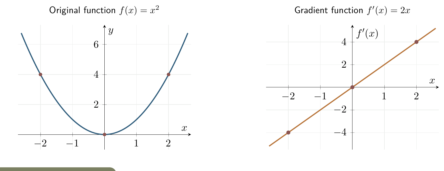
The derivative is not just a single number. If we differentiate a function, we obtain a new function that tells us the gradient everywhere.

Worked example 2: using a derivative function

For $f(x)=x^2$, the derivative is

\[f'(x)=2x.\]

Therefore:

Point	$x=-2$	$x=0$	$x=3$
Gradient $f'(x)$	-4	0	6

The derivative graph $y=f'(x)=2x$ records the tangent gradient of $y=f(x)=x^2$ at every $x$-value.

Graphs of f of x equals x squared and its derivative f prime of x equals 2x — The value of $f'(x)$ tells us the gradient of $f$ at the same $x$-coordinate.

Limits connect secants to a tangent

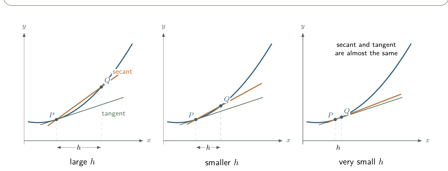
To estimate a curve's gradient at $x=a$, start with a second nearby point at $x=a+h$. The line joining the two points is a secant.

\[\text{secant gradient}=\frac{f(a+h)-f(a)}{h}.\]

As $h$ becomes smaller, the second point moves towards the first. The secant approaches the tangent, so the secant gradient approaches the derivative:

\[\boxed{f'(a)=\lim_{h\to0}\frac{f(a+h)-f(a)}{h}}.\]

Sequence of secant lines with smaller h approaching a tangent line — Large $h$ gives a visibly different secant. As $h\to0$, the secant line approaches the tangent.

Worked example 3: estimating the gradient of $f(x)=x^2$ at $x=1$

Use the secant-gradient expression with $a=1$:

\[ \frac{f(1+h)-f(1)}{h} =\frac{(1+h)^2-1}{h} =\frac{2h+h^2}{h} =2+h. \]

For smaller positive values of $h$, the gradients become:

$h$	1	0.5	0.1	0.01	0.001
Secant gradient $2+h$	3	2.5	2.1	2.01	2.001

The values approach 2, so $f'(1)=2$.

Video: What is a derivative?

Use this lesson to revisit the visual journey from secant gradients to the gradient of the tangent and the meaning of the derivative.

Finding a derivative at a point with the TI-Nspire CX

Technology can be used to evaluate a numerical derivative at a stated point. On calculator-allowed work, the TI-Nspire CX can evaluate $f'(a)$ directly; on non-calculator work, use the derivative information or differentiation rules available in the question.

Calculator method

Define or enter the function.
Use the numerical derivative command or derivative tool.
Evaluate the derivative at the required $x$-value.
Interpret the numerical result as the gradient of the tangent, with appropriate units when the variables have units.

Video: Derivative at any point on the TI-Nspire CX

The calculator tutorial demonstrates three practical ways of obtaining a derivative value and connects the output back to the tangent gradient.

The derivative as a rate of change

The same derivative idea applies whenever one quantity changes with respect to another. Gradient becomes a rate.

Simple rate model

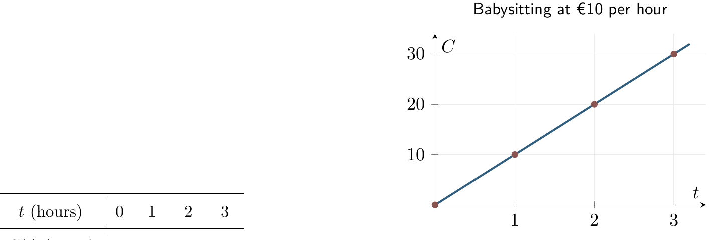
If a babysitter's total charge after $t$ hours is $C(t)=10t$ euros, then

\[C'(t)=10.\]

The derivative has units euros per hour, so the charge is increasing at a constant rate of €10 per hour.

Table and graph showing a babysitting cost increasing by 10 euros per hour — A constant derivative appears as a straight-line graph with constant gradient.

Worked example 4: average velocity approaching instantaneous velocity

A particle has displacement $s(t)=t^2$ metres. The average velocity from $t=3$ to $t=4$ is

\[\frac{s(4)-s(3)}{4-3}=\frac{16-9}{1}=7\text{ m/s}.\]

Now shorten the time interval:

Interval	[3,4]	[3,3.5]	[3,3.1]	[3,3.01]	[3,3.001]
Average velocity	7	6.5	6.1	6.01	6.001

As the second time approaches 3, the average velocity approaches $6\text{ m/s}$. Therefore the instantaneous velocity at $t=3$ is

\[s'(3)=6\text{ m/s}.\]

Derivative notation and units

The derivative can be written in several equivalent ways. The notation often reflects the variables in the problem.

Function or context	Derivative notation	Meaning
$y=f(x)$	$f'(x)$ or $\frac{dy}{dx}$	change in output per unit change in $x$
Displacement $s(t)$	$\frac{ds}{dt}$	velocity
Volume $V(r)$	$\frac{dV}{dr}$	change in volume per unit change in radius
Cost $C(q)$	$C'(q)$ or $\frac{dC}{dq}$	change in cost per unit change in quantity

Units of a derivative

Derivative units are

\[\frac{\text{units of the vertical quantity}}{\text{units of the horizontal quantity}}.\]

For example, if volume is measured in $\mathrm{cm^3}$ and radius in cm, then $dV/dr$ has units $\mathrm{cm^2}$.

Worked example 5: interpreting a derivative in context

Suppose $V(t)$ is the volume of water in a tank, in litres, after $t$ minutes, and

\[V'(12)=-3.5.\]

The negative sign means the volume is decreasing. The magnitude gives the rate.

Interpretation After 12 minutes, the volume of water is decreasing at $3.5\text{ L/min}$.

Two-part lesson summary

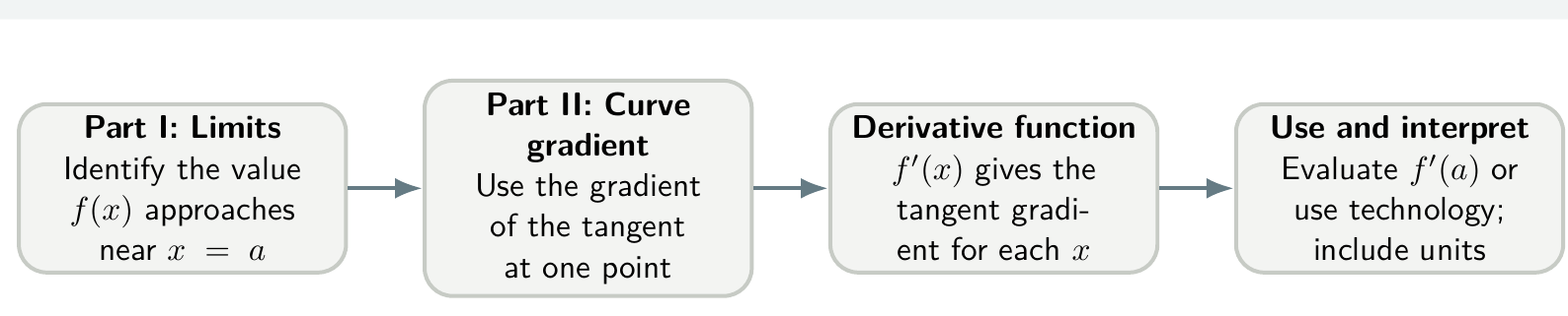
Summary diagram connecting limits, tangent gradients and rates of change — The lesson moves from approaching a value to approaching a tangent gradient, then interprets that derivative as a rate of change.

Part I: limits

A limit describes what outputs approach near an input value.
Approach from both sides for a two-sided limit.
The limit can differ from the actual function value.

Part II: derivatives

$f'(a)$ is the tangent gradient at $x=a$.
$f'(x)$ is the gradient function.
Derivative units are output-units per input-unit.

Practice

These questions follow the progression of the handout: limits first, then derivative meaning, secant gradients, calculator use and contextual interpretation.

A. Limits from tables and graphs

A table of values for $g(x)$ near $x=3$ approaches 5 from both sides. State $\lim_{x\to3}g(x)$.
As $x\to4^-$, $f(x)\to-1$, while as $x\to4^+$, $f(x)\to2$. Does $\lim_{x\to4}f(x)$ exist? Explain.
A graph has an open circle at $(2,6)$ and a filled point at $(2,1)$. State $\lim_{x\to2}f(x)$ and $f(2)$.
Use nearby values to estimate $\displaystyle\lim_{x\to1}\frac{x^2-1}{x-1}$.

B. Derivative and gradient

A graph passes through $(3,7)$, and the tangent at that point has gradient $-2$. State $f(3)$ and $f'(3)$.
Given $f'(x)=3x-4$, find the gradients of $f$ at $x=-2$, $x=0$ and $x=5$.
Explain the difference between $f(4)$ and $f'(4)$.
For $f(x)=x^2$, find the gradient of the secant joining the points with $x=2$ and $x=2.5$.
For $f(x)=x^2$, secant gradients from $x=2$ to $x=2+h$ approach 4 as $h\to0$. Estimate $f'(2)$.
Use a TI-Nspire numerical derivative to estimate $g'(2)$ for $g(x)=x^3-2x+1$. State the geometric meaning of your answer.

C. Rates and units

A car has displacement $s(t)$ km, where $t$ is in hours. Explain the meanings of $\frac{s(5)-s(3)}{5-3}$ and $s'(4)$.
$V'(8)=12$, where $V$ is volume in litres and $t$ is time in minutes. Interpret the statement.
$T'(15)=-0.7$, where $T$ is temperature in °C and time is in minutes. Interpret the statement.
If $V$ is measured in $\mathrm{cm^3}$ and $r$ in cm, give the units of $dV/dr$.
Revenue $R(t)$ is measured in dollars and $t$ in hours. Give the units of $R'(t)$, and explain what $R'(t)>0$ means.

Concise answer key

1. 5

2. No; the one-sided limits are different.

3. Limit = 6; $f(2)=1$.

4. 2

5. $f(3)=7$, $f'(3)=-2$.

6. $-10,-4,11$.

7. $f(4)$ is the output; $f'(4)$ is the tangent gradient.

8. 4.5

9. 4

10. $g'(2)=10$; the tangent gradient is 10.

11. Average velocity from 3 h to 5 h; instantaneous velocity at 4 h, both in km/h.

12. Volume increasing at 12 L/min.

13. Temperature decreasing at 0.7 °C/min.

14. $\mathrm{cm^2}$.

15. $/h; revenue is increasing.

Function or context	Derivative notation	Meaning
\(y=f(x)\)	\(f'(x)\) or \(\frac{dy}{dx}\)	change in output per unit change in \(x\)
Displacement \(s(t)\)	\(\frac{ds}{dt}\)	velocity
Volume \(V(r)\)	\(\frac{dV}{dr}\)	change in volume per unit change in radius
Cost \(C(q)\)	\(C'(q)\) or \(\frac{dC}{dq}\)	change in cost per unit change in quantity

Contact / enquiry