IB Mathematics: Analysis and Approaches HL — Topic 5 Calculus
Limits, Continuity and First Principles
Connect secant gradients to tangent gradients, understand continuity and differentiability, and derive derivatives from the limit definition.
Learning goal
Understand limits, continuity and differentiability informally; use the derivative definition from first principles for polynomial functions; and interpret and calculate higher derivatives.
Syllabus link
AHL 5.12 Informal continuity and differentiability, convergence and divergence of limits, first-principles differentiation for polynomials, and higher-derivative notation.
Big idea
A derivative is not an isolated rule: it is the limit of secant gradients as two points on a curve move together. Higher derivatives then describe how rates of change themselves change.
Key definition
\(\displaystyle f'(x)=\lim_{h\to0}\frac{f(x+h)-f(x)}h\).
Why do we need limits?
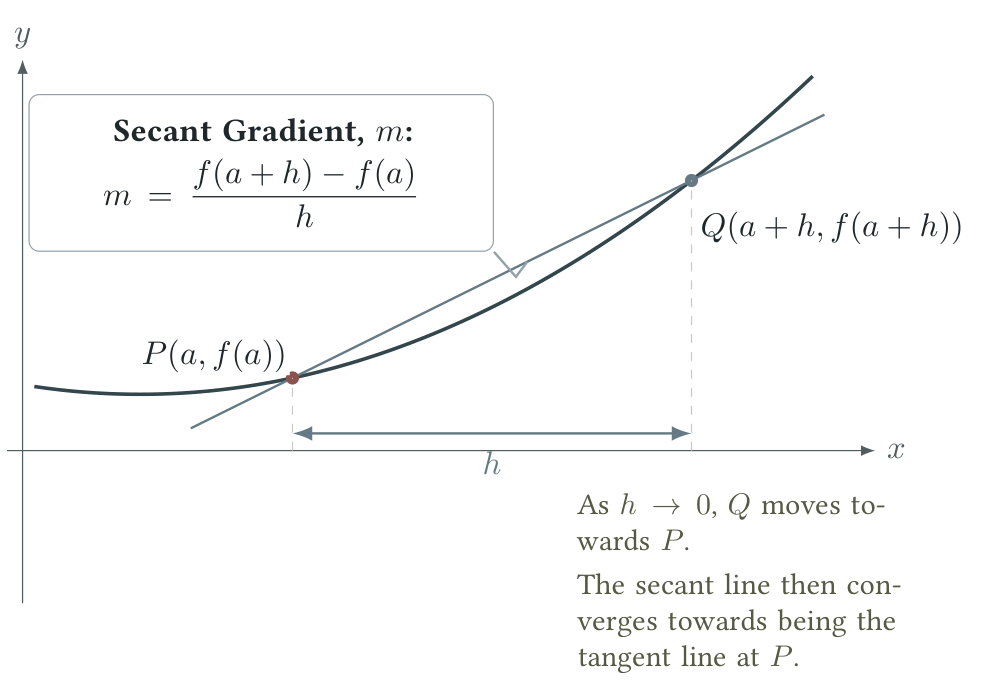
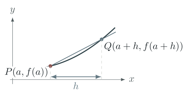
A derivative asks for the gradient of a tangent at one point. However, a gradient normally needs two points. Limits solve this problem: we begin with a secant through two nearby points, then study what its gradient approaches as the second point moves towards the first.
This opening section introduces the key idea. We will return to this illustration in Section 5, where we use limits to turn the secant-gradient expression into the definition of the derivative function from first principles.
Key idea
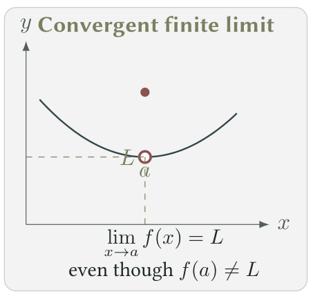
A limit describes the value that an expression approaches. The expression does not necessarily have to equal that value at the point itself.
means that the values of \(f(x)\) can be made as close as we like to \(L\) by taking \(x\) sufficiently close to \(a\).
Limits: convergence and divergence
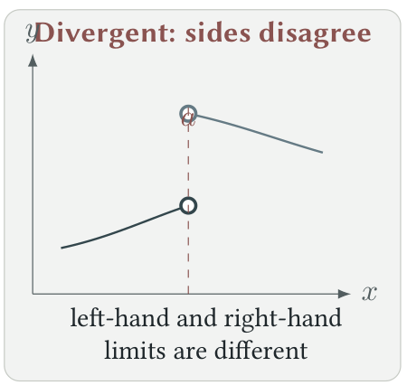
A limit converges when the function approaches one finite value. It diverges when there is no single finite value being approached.
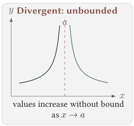
Reading a two-sided limit
For \(\lim\limits_{x\to a}f(x)\) to converge to \(L\), both one-sided approaches must agree:
The actual value \(f(a)\) is a separate question.
Worked example 1: a polynomial limit
Evaluate
Solution
Polynomials are continuous everywhere, so direct substitution is valid:
Answer:
Worked example 2: interpreting a graph
Suppose a graph approaches \(4\) from both sides as \(x\to 1\), but the plotted point at \(x=1\) is \((1,7)\). State the limit and the actual function value.
Solution
Then
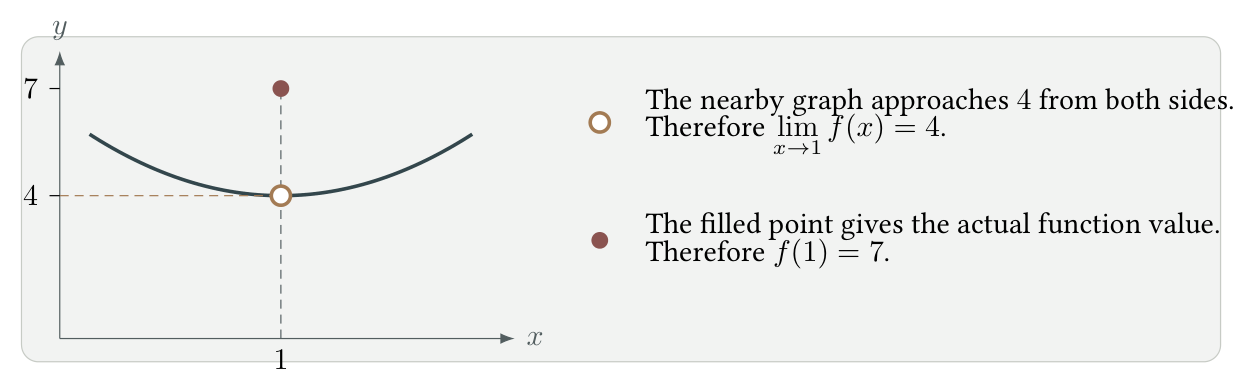
The limit records the nearby behaviour, not the isolated plotted value.
Continuity: an informal picture
Informally, a function is continuous at \(x=a\) when there is no break, jump or hole there. Close to \(a\), the graph approaches the same height as the actual point on the graph.
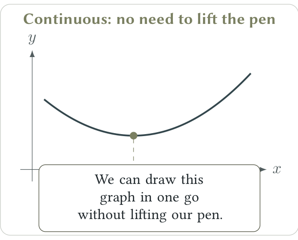
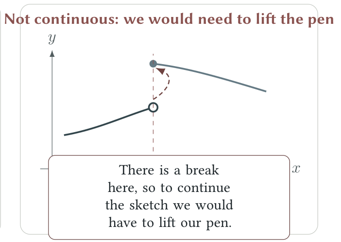
A very useful classroom picture is this: if we can draw the graph without lifting our pen from the paper, then we think of the function as continuous. If we would have to lift our pen because there is a hole, a jump or some other break, then the function is not continuous.
Continuity at a point - informal understanding
A useful picture is
We use this as an interpretation, not as a formal continuity test. In AHL 5.12, formal examination questions asking us to test continuity or differentiability are not required.
The two sketches below illustrate this pen-test idea. In the first sketch, we can trace the graph in one continuous stroke without lifting our pen. In the second sketch, there is a break in the graph, so we would have to lift our pen to continue drawing it.
Syllabus focus
We need to recognise and discuss continuity and differentiability informally, but the syllabus states that examination questions will not ask us to carry out formal tests for them.
Differentiability: does one tangent gradient exist?
A function is differentiable at a point when the tangent gradient there is unique and finite. Every differentiable function is continuous at that point, but a continuous graph can still fail to be differentiable.
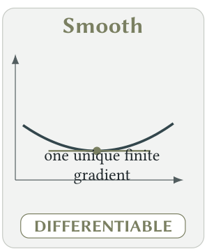
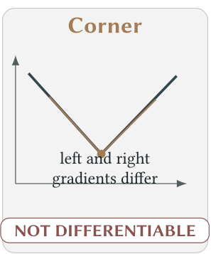
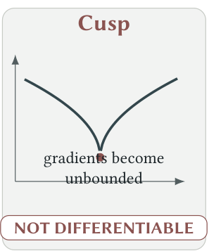
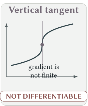
Conclusion. Only the smooth graph is differentiable at the marked point. The corner, cusp and vertical tangent are all continuous there, but they are not differentiable because there is no unique finite tangent gradient.
Worked example 3: why \(|x|\) is not differentiable at \(x=0\)
Explain why \(f(x)=|x|\) is continuous but not differentiable at \(x=0\).
Solution
For \(f(x)=|x|\), the graph is continuous at the origin. However,
The illustration below makes the mismatch clear.
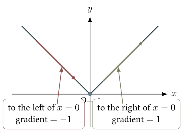
Because the two one-sided gradients do not agree, there is no unique tangent gradient at \(x=0\). The function is continuous there, but not differentiable there.
From secants to the derivative from first principles
We now return to the illustration from Section 1. Recall that to find the derivative we begin with the gradient of a secant line through two points on the curve, and then we study what happens as the second point moves towards the first.
Let \(P=(a,f(a))\) and \(Q=(a+h,f(a+h))\). The secant gradient is
As \(h\to 0\), the point \(Q\) moves towards \(P\). If the secant gradients approach a finite value, the secant approaches the tangent.
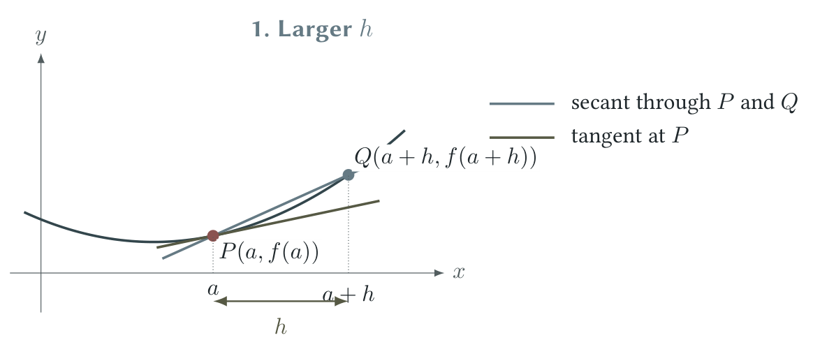
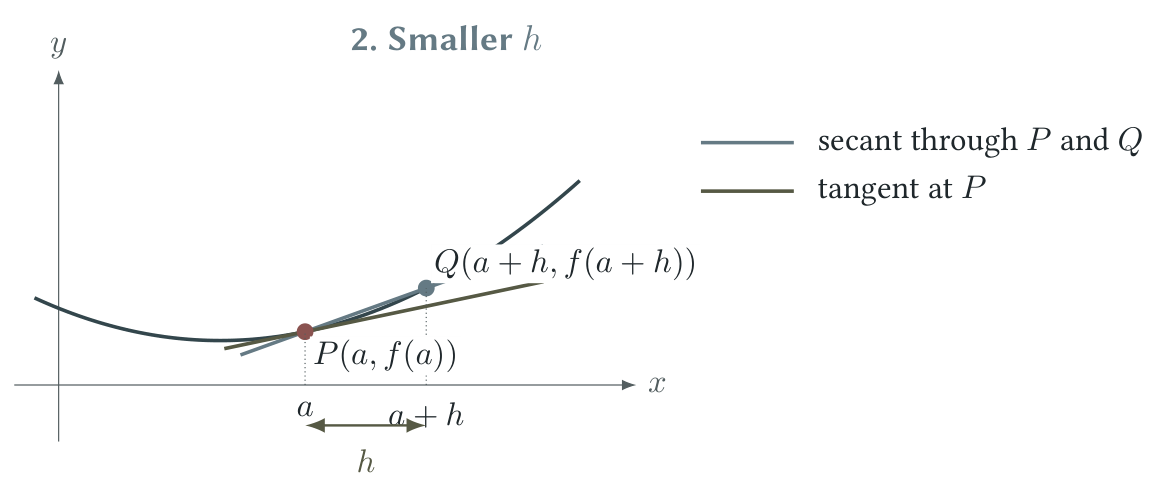
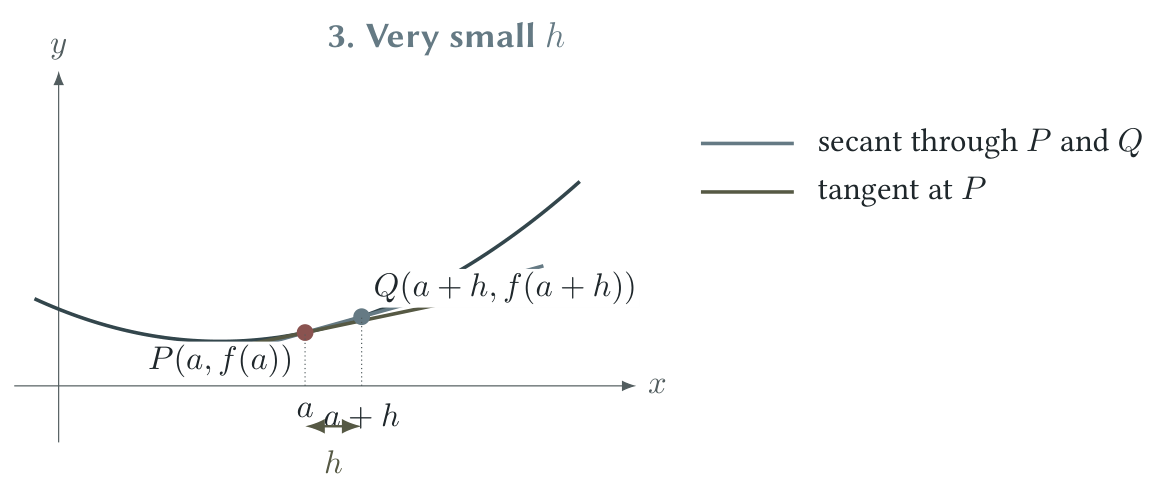
Successive secants as \(h\) gets smaller
What the progression shows
In all three sketches, the secant gradient is
As \(h\) gets smaller and smaller, point \(Q\) moves closer and closer to point \(P\). At the same time, the secant line through \(P\) and \(Q\) gets closer and closer to the tangent to the curve at \(P\).
In the limit, we let \(h\to 0\) (without ever starting by substituting \(h=0\) into the fraction), so the secant gradient approaches the tangent gradient:
The expression \(\displaystyle \frac{f(x+h)-f(x)}{h}\) is the difference quotient.
Definition of the derivative
This is the derivative from first principles. In this syllabus section, we use the definition for polynomial functions.
Differentiation from First Principles
Use this tutorial alongside the derivation below to see how the difference quotient becomes the derivative, with the algebra written out carefully.
Common trap
We never substitute \(h=0\) into the difference quotient at the start: that would produce division by zero. First simplify until the factor \(h\) cancels; only then evaluate the limit as \(h\to 0\).
A reliable first-principles method
Four algebraic moves
To find \(f'(x)\) from first principles:
Write \(f(x+h)\) carefully.
Form \(f(x+h)-f(x)\) and expand.
Factor out and cancel the common factor \(h\).
Evaluate the remaining limit as \(h\to 0\).
| Expression | Algebraic move |
|---|---|
| \(f(x+h)\) | Substitute \(x+h\) |
| \(f(x+h)-f(x)\) | Expand brackets |
| \(h(\cdots)\) | Factor and cancel \(h\) |
| \(h\to0\) | Evaluate the limit |
Worked example 4: derive the derivative of \(f(x)=x^2\)
Use first principles to derive the derivative of \(f(x)=x^2\).
Solution
Starting from the definition,
Answer: \(f'(x)=2x\)
Worked example 5: derive the derivative of \(f(x)=2x^3-5x+1\)
Use first principles to derive the derivative of \(f(x)=2x^3-5x+1\).
Solution
Answer: \(f'(x)=6x^2-5\)
First principles at a particular point
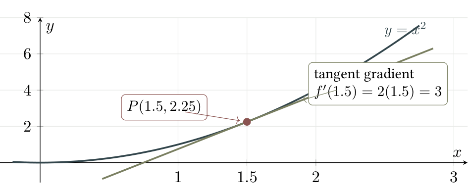
We can either derive a general expression for \(f'(x)\) and then substitute the required \(x\)-value, or use the point form directly:
Worked example 6: tangent gradient at a point
Use first principles to find the gradient of \(f(x)=x^2-4x+1\) at \(x=3\).
Solution
Here \(a=3\), so
Now
and \(f(3)=9-12+1=-2\). Therefore
Answer: The tangent gradient at \(x=3\) is \(2\).
Three common first-principles errors
| Error | How to avoid it |
|---|---|
| Substituting \(h=0\) too early | This gives \(0/0\). Simplify and cancel \(h\) first. |
| Expanding \(f(x+h)\) incorrectly | Every occurrence of \(x\) must be replaced by \((x+h)\), with brackets. |
| Forgetting to subtract all of \(f(x)\) | Write \(-[f(x)]\) with brackets before expanding signs. |
A useful check
Once we have found a derivative by first principles, we can check it using the familiar differentiation rules. The first-principles derivation explains why those rules work; the rules then provide efficiency.
Higher derivatives
The first derivative measures the rate of change of \(f\). The second derivative measures the rate of change of \(f'\), and so on.
| Derivative | Meaning | Next step |
|---|---|---|
| \(f(x)\) | Original quantity | Differentiate |
| \(f'(x)\) | Rate of change | Differentiate |
| \(f''(x)\) | Change in the rate | Repeat |
| \(f^{(n)}(x)\) | \(n\)th derivative |
How to read higher-derivative notation aloud
Each successive derivative can be read in both prime notation and Leibniz notation:
- \[\displaystyle f'(x)=\frac{dy}{dx}\]
is read as “\(f\) prime of \(x\)” or “dee \(y\) by dee \(x\)”.
- \[\displaystyle f''(x)=\frac{d^2y}{dx^2}\]
is read as “\(f\) double prime of \(x\)” or “dee squared \(y\) by dee \(x\) squared”.
- \[\displaystyle f^{(3)}(x)=\frac{d^3y}{dx^3}\]
is read as “the third derivative of \(f\)” or “dee cubed \(y\) by dee \(x\) cubed”.
- \[\displaystyle f^{(n)}(x)=\frac{d^ny}{dx^n}\]
is read as “the \(n\)th derivative of \(f\)” or “dee to the \(n\) \(y\) by dee \(x\) to the \(n\)”.
Important: \(\dfrac{d^2y}{dx^2}\) means the second derivative of \(y\) with respect to \(x\); it does not mean \(\left(\dfrac{dy}{dx}\right)^2\).
Seeing \(f\), \(f'\) and \(f''\) together
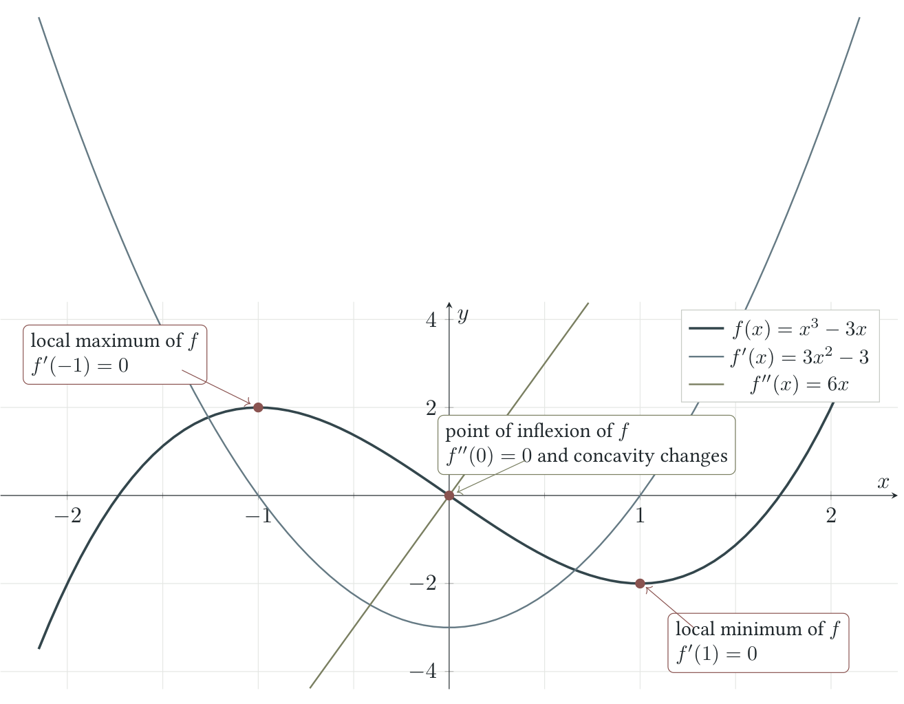
Consider
How to read the three graphs together
At any chosen value of \(x\), imagine drawing a vertical line through the three graphs.
The height of \(f'(x)\) tells us the gradient of \(f\) at that same \(x\)-value.
The sign of \(f''(x)\) tells us the concavity of \(f\): when \(f''(x)<0\), the curve is concave down, and when \(f''(x)>0\), the curve is concave up. When this is combined with the sign of \(f'(x)\), we can also tell whether the curve is getting steeper or becoming less steep.
We now read the picture systematically from left to right along the \(x\)-axis.
First read \(f'\) from left to right
For \(x<-1\): the graph of \(f'\) lies above the \(x\)-axis, so \(f'(x)>0\). Therefore the graph of \(f\) is increasing.
At \(x=-1\): the graph of \(f'\) crosses the \(x\)-axis, so \(f'(-1)=0\). The sign of \(f'\) changes from positive to negative, so \(f\) changes from increasing to decreasing. Therefore \(f\) has a local maximum at
\[(-1,f(-1))=(-1,2).\]For \(-1<x<1\): the graph of \(f'\) lies below the \(x\)-axis, so \(f'(x)<0\). Therefore the graph of \(f\) is decreasing. Notice that \(f'\) reaches its lowest value at \(x=0\), where \(f'(0)=-3\). This is where \(f\) has its most negative tangent gradient and is decreasing most steeply.
At \(x=1\): the graph of \(f'\) crosses the \(x\)-axis again, so \(f'(1)=0\). The sign of \(f'\) changes from negative to positive, so \(f\) changes from decreasing to increasing. Therefore \(f\) has a local minimum at
\[(1,f(1))=(1,-2).\]For \(x>1\): the graph of \(f'\) lies above the \(x\)-axis, so \(f'(x)>0\). Therefore the graph of \(f\) is increasing again.
Now read \(f''\) and the concavity of \(f\) from left to right
The sign of \(f''\) tells us whether the graph of \(f\) is concave down or concave up. To describe whether the curve is getting steeper or becoming less steep, we combine this with what we already know from the sign of \(f'\).
For \(x<-1\): the graph of \(f''\) lies below the \(x\)-axis, so \(f''(x)<0\) and the graph of \(f\) is concave down. We already know that \(f'(x)>0\) here, so \(f\) is increasing; however, the curve becomes less and less steep as it approaches the local maximum at \(x=-1\).
For \(-1<x<0\): we still have \(f''(x)<0\), so the graph of \(f\) remains concave down. Now \(f'(x)<0\), so \(f\) is decreasing, and the curve becomes steeper and steeper downwards as it approaches \(x=0\).
At \(x=0\): we have \(f''(0)=0\), and the sign of \(f''\) changes from negative to positive. The graph of \(f\) changes from concave down to concave up, so
\[(0,f(0))=(0,0)\]is a point of inflexion. At this point, the curve has its steepest downward tangent because \(f'(0)=-3\) is the minimum value of \(f'\).
For \(0<x<1\): the graph of \(f''\) lies above the \(x\)-axis, so \(f''(x)>0\) and the graph of \(f\) is concave up. Since \(f'(x)<0\), the curve is still decreasing, but it becomes less and less steep as it approaches the local minimum at \(x=1\).
For \(x>1\): we still have \(f''(x)>0\), so the graph of \(f\) remains concave up. Here \(f'(x)>0\), so the curve is increasing and becomes steeper and steeper as \(x\) increases.
Putting the information from \(f'\) and \(f''\) together
| Interval | Sign of \(f'\) | Sign of \(f''\) | What we see on the graph of \(f\) |
|---|---|---|---|
| \(x<-1\) | + | − | \(f\) is increasing and concave down: the curve rises but becomes less steep as it approaches the local maximum. |
| \(-1<x<0\) | − | − | \(f\) is decreasing and concave down: the curve falls increasingly steeply towards the point of inflexion. |
| \(0<x<1\) | − | + | \(f\) is decreasing and concave up: the curve continues to fall but becomes less steep as it approaches the local minimum. |
| \(x>1\) | + | + | \(f\) is increasing and concave up: the curve rises and becomes increasingly steep. |
The central relationship
The graph of \(f'\) records the gradient of \(f\). The sign of \(f''\) tells us whether the graph of \(f\) is concave down or concave up. Reading the signs of \(f'\) and \(f''\) together tells us whether the curve is increasing or decreasing, how it bends, and whether it is getting steeper or becoming less steep.
Worked example 7: repeated differentiation
Let \(f(x)=2x^6-3x^4+5x-7\). Find \(f^{(4)}(x)\).
Solution
Answer: \(f^{(4)}(x)=720x^2-72\)
Higher derivatives in motion: kinematics
As we have already seen in IB Mathematics AA syllabus section SL 5.9: Kinematics, motion can be described using displacement \(s\), velocity \(v\) and acceleration \(a\). We now return to those relationships and view them through the language of higher derivatives.
When \(s(t)\) is displacement, velocity is the first derivative of displacement and acceleration is the second derivative of displacement:
| Quantity | Notation and units | Relationship |
|---|---|---|
| Displacement | \(s(t)\) in metres | Differentiate with respect to \(t\) to find velocity. |
| Velocity | \(v(t)=s'(t)\) in \(\mathrm{m\,s}^{-1}\) | Differentiate again to find acceleration. |
| Acceleration | \(a(t)=s''(t)\) in \(\mathrm{m\,s}^{-2}\) | Second derivative of displacement. |
Worked example 8: displacement, velocity and acceleration
A particle has displacement
Find its velocity and acceleration, then determine the acceleration at \(t=2\).
Solution
Therefore
Answer: \(v(t)=3t^2-12t+9\), \(a(t)=6t-12\), and \(a(2)=0\) m s\(^{-2}\).
Practice
Evaluate \(\displaystyle \lim_{x\to -2}(2x^4-3x^2+5x-1)\).
A graph approaches \(3\) as \(x\to 4\) from the left and \(-1\) as \(x\to 4\) from the right. State whether \(\displaystyle\lim_{x\to 4}f(x)\) converges or diverges, and explain why.
A graph has an open circle at \((2,5)\) and a filled point at \((2,1)\). From both sides, the graph approaches the open circle. State \(\displaystyle\lim_{x\to 2}f(x)\) and \(f(2)\). Is the function continuous at \(x=2\)?
Explain why continuity at a point does not guarantee differentiability there. Give one graphical feature that illustrates this.
Use first principles to derive the derivative of \(f(x)=3x+7\).
Use first principles to derive the derivative of \(f(x)=x^2+4x-2\).
Use first principles to derive the derivative of \(f(x)=x^3-2x\).
Use first principles to find the gradient of \(f(x)=2x^2-x+3\) at \(x=1\).
Let \(f(x)=5x^7-2x^5+3x^2-4\). Find \(f'(x)\), \(f''(x)\) and \(f^{(3)}(x)\).
For \(g(x)=x^8\), write a general expression for \(g^{(n)}(x)\) for \(0\le n\le 8\). Hence find \(g^{(8)}(x)\).
A particle has displacement \(s(t)=2t^4-5t^3+3t\). Find \(v(t)\) and \(a(t)\), and calculate \(a(1)\).
The following claims are made. Decide whether each is true or false, and justify your answer.
If \(f\) is differentiable at \(x=a\), then it is continuous at \(x=a\).
If \(f\) is continuous at \(x=a\), then it is differentiable at \(x=a\).
If \(\lim_{x\to a}f(x)=L\), then \(f(a)\) must equal \(L\).
If the left-hand and right-hand limits are different, the two-sided limit diverges.
Answer key
1. Polynomial limit
2. One-sided limits
The limit diverges because
A two-sided limit can converge only when the two one-sided limits agree.
3. Hole and separate function value
The function is not continuous at \(x=2\) because the limiting value and the actual function value are different.
4. Continuity versus differentiability
A continuous graph may still have no unique finite tangent gradient. A corner, cusp or vertical tangent is enough to make the function non-differentiable at that point. For example, \(f(x)=|x|\) is continuous at \(0\) but has left gradient \(-1\) and right gradient \(+1\).
5. \(f(x)=3x+7\) from first principles
6. \(f(x)=x^2+4x-2\) from first principles
7. \(f(x)=x^3-2x\) from first principles
8. Gradient at \(x=1\)
First principles gives \(f'(x)=4x-1\). Therefore
The gradient is \(3\).
9. Higher derivatives
10. The \(n\)th derivative of \(x^8\)
For \(0\le n\le 8\),
Hence
11. Motion
Thus
12. True or false
True. Differentiability at a point implies continuity there.
False. A continuous function can have a corner, cusp or vertical tangent.
False. The limit describes nearby behaviour; the function value may be different or undefined.
True. A two-sided limit requires the two one-sided limits to agree.