IB Mathematics: Analysis and Approaches HL — Topic 5 Calculus
First-Order Differential Equations
Recognise the structure of a first-order differential equation, choose the correct exact or numerical method, and interpret solutions in mathematical and real-world contexts.
Learning goal
Solve separable, homogeneous and linear first-order equations, then approximate solutions numerically with Euler’s method.
Syllabus link
AHL 5.18 Separable and homogeneous equations, integrating factors, logistic growth and Euler’s method.
Big idea
A differential equation gives a rule for change. Its structure tells you which method will turn that rule into a usable solution.
Key relationships
\(y=vx\), \(\mu=e^{\int P(x)\,dx}\), and \(y_{n+1}=y_n+h f(x_n,y_n)\).
Language and structure of differential equations
A differential equation is an equation whose unknown is a function. It links that unknown function to one or more derivatives, so its solutions are curves rather than isolated numbers.
Worked example 1: verify a proposed solution
Show that \(y=3e^{2x}-\frac{x}{2}-\frac14\) solves \(y'-2y=x\).
Differentiate:
\[y'=6e^{2x}-\frac12.\]Now substitute both \(y\) and \(y'\) into the differential equation:
\[\begin{aligned}y'-2y&=\left(6e^{2x}-\frac12\right)-2\left(3e^{2x}-\frac{x}{2}-\frac14\right)\\&=6e^{2x}-\frac12-6e^{2x}+x+\frac12\\&=x.\end{aligned}\]The left side becomes the right side for every permitted \(x\), so the function is a solution.
Verification means an identity
Checking one numerical value is not enough. Substitute the proposed function and its derivative and show that the differential equation holds throughout the interval.
Separable differential equations
An equation is separable when it can be rearranged into \(G(y)\,dy=H(x)\,dx\), after which both sides can be integrated.
Separation method
- Move every factor involving \(y\) with \(dy\), and every factor involving \(x\) with \(dx\).
- Integrate both sides and include one arbitrary constant.
- Use the initial condition when one is given.
- Make \(y\) the subject when possible and state relevant domain restrictions.
Separable Differential Equations
The complete separation-of-variables process: rearrange, integrate and use a condition to determine the constant.
Worked example 2: inverse-trigonometric integral
Solve \(\frac{dy}{dx}=3x^2(1+y^2)\), with \(y(0)=1\).
\[\frac1{1+y^2}\,dy=3x^2\,dx.\]\[\int\frac1{1+y^2}\,dy=\int3x^2\,dx\quad\Longrightarrow\quad\arctan y=x^3+C.\]From \(y(0)=1\), \(C=\pi/4\). Hence
\[\boxed{y=\tan\!\left(x^3+\frac\pi4\right)}.\]The formula is valid on any interval containing \(x=0\) on which the tangent expression is defined.
Worked example 3: separation leading to a logarithm
Solve \(\frac{dy}{dx}=(x+1)e^{-y}\), with \(y(0)=0\).
\[e^y\frac{dy}{dx}=x+1\quad\Longrightarrow\quad \int e^y\,dy=\int(x+1)\,dx.\]\[e^y=\frac{x^2}2+x+C.\]The condition gives \(C=1\), so
\[\boxed{y=\ln\!\left(\frac{x^2}2+x+1\right)}.\]Since \(\frac12[(x+1)^2+1]>0\), the logarithm is defined for every real \(x\).
Equilibrium solutions can be lost during division
Before dividing by a factor involving the dependent variable, check whether that factor can be zero. Those values can produce constant equilibrium solutions that division would erase.
Worked example 4: complete logistic-type solution set
Find all solutions of \(y'=y(3-y)\).
Partial fractions give \(\frac1{y(3-y)}=\frac13\left(\frac1y+\frac1{3-y}\right)\). Hence
\[\frac13\bigl(\ln|y|-\ln|3-y|\bigr)=x+C\quad\Longrightarrow\quad\frac{y}{3-y}=Ce^{3x}.\]Solving for \(y\):
\[\boxed{y=\frac{3Ce^{3x}}{1+Ce^{3x}}},\qquad C\neq0.\]The complete solution set is the two equilibrium solutions together with this non-equilibrium family.
Common separation trap
Always check for constant solutions before dividing by a \(y\)-factor.
The logistic equation
A standard logistic model is
\[\frac{dn}{dt}=kn(a-n),\qquad a>0.\]The constant \(a\) is the carrying capacity: the population level supported in the long run by the modelled environment. The equilibrium solutions are \(n=0\) and \(n=a\). For non-equilibrium solutions, separation gives
\[\boxed{n(t)=\frac{a}{1+Ce^{-akt}}},\qquad C=\frac{a-n_0}{n_0}\text{ if }n(0)=n_0.\]Worked example 5: exact logistic model
\(P' =0.0005P(1200-P)\), \(P(0)=100\). Find \(P(t)\), then find when \(P=900\).
Here \(a=1200\), \(k=0.0005\), so \(ak=0.6\), and \(C=(1200-100)/100=11\). Therefore
\[\boxed{P(t)=\frac{1200}{1+11e^{-0.6t}}}.\]Set \(P=900\):
\[900=\frac{1200}{1+11e^{-0.6t}}\Longrightarrow e^{-0.6t}=\frac1{33}\Longrightarrow \boxed{t=\frac{\ln33}{0.6}\approx5.83}.\]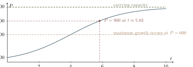
Homogeneous differential equations: use \(y=vx\)
In AHL 5.18, a first-order homogeneous differential equation can be written as
\[\frac{dy}{dx}=F\!\left(\frac yx\right).\]Rewrite the whole right-hand side in terms of \(y/x\). Then set \(v=y/x\), so \(y=vx\) and, crucially,
\[\boxed{\frac{dy}{dx}=v+x\frac{dv}{dx}}.\]Homogeneous-equation method
- Confirm the right-hand side depends only on \(y/x\).
- Set \(v=y/x\), so \(y=vx\) and \(y'=v+xv'\).
- Substitute and rearrange to obtain a separable equation in \(v\) and \(x\).
- Integrate, replace \(v\) by \(y/x\), then apply any condition.
Worked example 6: homogeneous equation with explicit solution
Solve \(y'=y/x+x/y\), \(y(1)=2\), for \(x>0\), \(y>0\).
The right side is \(y/x+1/(y/x)\), so set \(v=y/x\). Then
\[v+x\frac{dv}{dx}=v+\frac1v\quad\Longrightarrow\quad v\,dv=\frac1x\,dx.\]\[\frac{v^2}2=\ln x+C\quad\Longrightarrow\quad v^2=2\ln x+C_1.\]Replace \(v=y/x\) and use \(y(1)=2\): \(C_1=4\). Thus
\[y^2=x^2(2\ln x+4).\]Because \(y(1)>0\), choose the positive branch:
\[\boxed{y=x\sqrt{2\ln x+4}}.\]Worked example 7: implicit homogeneous solution
Solve \(y'=(x+y)/(x-y)\).
Divide numerator and denominator by \(x\), then set \(v=y/x\):
\[v+xv'=\frac{1+v}{1-v}\quad\Longrightarrow\quad xv'=\frac{1+v^2}{1-v}.\]\[\frac{1-v}{1+v^2}\,dv=\frac1x\,dx.\]Integrating gives
\[\arctan v-\frac12\ln(1+v^2)=\ln|x|+C.\]After substituting \(v=y/x\) and simplifying the logarithms, the \(\ln|x|\) terms cancel:
\[\boxed{\arctan\!\left(\frac yx\right)-\frac12\ln(x^2+y^2)=C}.\]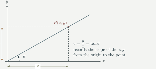
The product-rule term is essential
Because \(v\) changes with \(x\), differentiating \(y=vx\) gives \(y'=v+xv'\), not \(y'=xv'\).
Homogeneous Differential Equations
Recognise dependence on y/x, use y=vx, apply the product rule and reduce the equation to a separable form.
Linear first-order equations and integrating factors
Write a linear first-order equation in standard form
\[\boxed{y'+P(x)y=Q(x)}.\]The coefficient of \(y'\) must be 1. Then use
\[\boxed{\mu(x)=e^{\int P(x)\,dx}},\qquad \boxed{(\mu y)'=\mu Q},\qquad \boxed{y=\frac1\mu\left(\int\mu Q\,dx+C\right)}.\]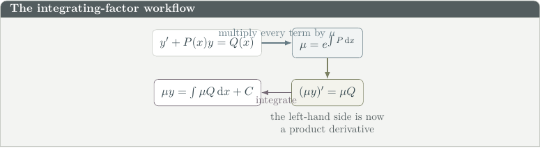
Five-step method
- Put the equation into \(y'+P(x)y=Q(x)\).
- Find \(\mu=e^{\int P(x)dx}\).
- Multiply every term by \(\mu\).
- Replace the left side by \((\mu y)'\).
- Integrate, solve for \(y\), then use any initial condition.
Linear Differential Equation 1
Introduce the standard linear form and the integrating-factor method before the first complete example.
Worked example 8: constant coefficient
Solve \(y'+2y=e^x\), \(y(0)=3\).
Here \(P(x)=2\), so \(\mu=e^{2x}\). Multiply by \(e^{2x}\):
\[e^{2x}y'+2e^{2x}y=e^{3x}\quad\Longrightarrow\quad(e^{2x}y)'=e^{3x}.\]\[e^{2x}y=\frac13e^{3x}+C\quad\Longrightarrow\quad y=\frac13e^x+Ce^{-2x}.\]Using \(y(0)=3\) gives \(C=8/3\):
\[\boxed{y=\frac13e^x+\frac83e^{-2x}}.\]Linear Differential Equation 2
A second guided example reinforcing P(x), the integrating factor, the product derivative and the initial condition.
Worked example 9: first put the equation in standard form
Solve \(xy'-2y=x^3\), \(y(1)=4\), for \(x>0\).
Divide the entire equation by \(x\): \(y'-\frac2x y=x^2\). Therefore
\[\mu=e^{\int-2/x\,dx}=e^{-2\ln x}=x^{-2}.\]Multiplying through gives \((x^{-2}y)'=1\), so
\[x^{-2}y=x+C\quad\Longrightarrow\quad y=x^3+Cx^2.\]Use \(y(1)=4\): \(C=3\). Hence
\[\boxed{y=x^3+3x^2}.\]Linear Differential Equation 3
Consolidate the full method after an equation whose y-prime coefficient was not initially 1.
Newton’s law of cooling
If the ambient temperature \(T_a\) is constant,
\[\frac{dT}{dt}=-k(T-T_a),\qquad k>0,\]with solution
\[\boxed{T(t)=T_a+(T_0-T_a)e^{-kt}}.\]Worked example 10: cooling model
A drink is initially \(90^\circ\mathrm C\) in a \(20^\circ\mathrm C\) room. After 10 minutes it is \(55^\circ\mathrm C\). When does it reach \(30^\circ\mathrm C\)?
The model is \(T=20+70e^{-kt}\). From \(T(10)=55\):
\[35=70e^{-10k}\Longrightarrow e^{-10k}=\frac12\Longrightarrow k=\frac{\ln2}{10}.\]Now set \(T=30\):
\[10=70e^{-kt}\Longrightarrow e^{-kt}=\frac17\Longrightarrow \boxed{t=\frac{10\ln7}{\ln2}\approx28.1\text{ min}}.\]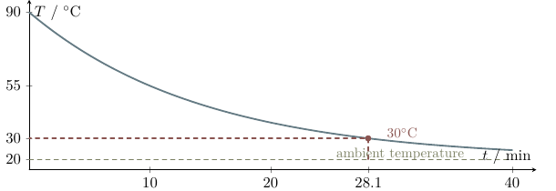
Why the integrating factor works
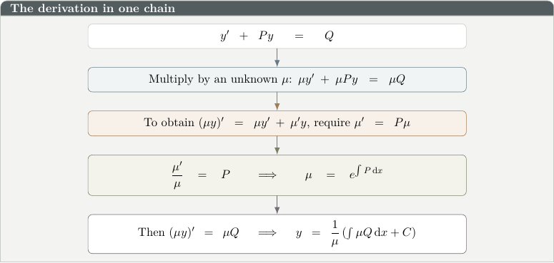
After multiplying \(y'+Py=Q\) by an unknown \(\mu\), the left side is \(\mu y'+\mu Py\). To make this exactly \((\mu y)'=\mu y'+\mu' y\), require \(\mu'=P\mu\). Therefore \(\mu'/\mu=P\), so \(\ln|\mu|=\int P\,dx\) and the convenient choice is \(\mu=e^{\int Pdx}\).
Euler’s method
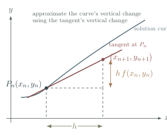
Euler’s method builds an approximate solution to \(y'=f(x,y)\) from an initial point \((x_0,y_0)\) and a fixed step size \(h\).
At the current point \(P_n=(x_n,y_n)\), the differential equation gives the tangent gradient \(f(x_n,y_n)\). Moving horizontally by \(h\), the tangent predicts a vertical change \(h f(x_n,y_n)\). That tangent step is used as the next approximate point.
The most important Euler rule
Evaluate the gradient at the current point first. Do not update \(y\) and then use the new value in the slope for the same step.
Worked example 11: build \(P_1,P_2,P_3\) step by step
Use Euler’s method with \(h=0.2\) to estimate \(y(0.6)\) for \(y'=x+y\), \(y(0)=1\).
Hence
\[\boxed{y(0.6)\approx1.856}.\]The exact solution is \(y=2e^x-x-1\), giving \(y(0.6)\approx2.044\). The Euler estimate is lower because the solution curve bends upward while each tangent segment lies below it after the point of contact.
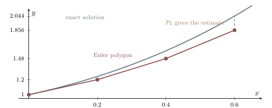
| \(n\) | \(x_n\) | \(y_n\) | Current slope \(x_n+y_n\) | Updated \(y_{n+1}\) |
|---|---|---|---|---|
| 0 | 0.0 | 1.000 | 1.000 | 1.200 |
| 1 | 0.2 | 1.200 | 1.400 | 1.480 |
| 2 | 0.4 | 1.480 | 1.880 | 1.856 |
Worked example 12: numerical logistic growth
\(P\), measured in thousands, satisfies \(P'=0.4P(1-P/10)\), \(P(0)=2\). Use Euler’s method with \(h=0.5\) to estimate \(P(1.5)\).
| \(n\) | \(t_n\) | \(P_n\) | \(f(t_n,P_n)\) | \(P_{n+1}\) |
|---|---|---|---|---|
| 0 | 0.0 | 2.0000 | 0.6400 | 2.3200 |
| 1 | 0.5 | 2.3200 | 0.712704 | 2.676352 |
| 2 | 1.0 | 2.676352 | ≈0.784026 | 3.068365 |
Thus \(\boxed{P(1.5)\approx3.07\text{ thousand}}\), approximately 3070 people.
Technology note
A spreadsheet can generate an Euler table efficiently: enter \(x_n\), \(y_n\), the current slope \(f(x_n,y_n)\), then the update formula in the next row. Keep the initial value, step size, current slope and new value clearly visible.
Euler’s Method for Differential Equations — TI-Nspire CX
Connect the hand-built Euler table to an efficient graphical-calculator implementation.
Choosing the correct method
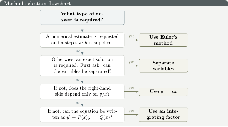
Four high-frequency errors
- Euler: using the updated \(y\) too early or taking the wrong number of steps.
- Separable: losing equilibrium solutions by division or forgetting the constant of integration.
- Homogeneous: writing \(y'=xv'\) instead of \(y'=v+xv'\).
- Linear: finding the integrating factor before first making the coefficient of \(y'\) equal to 1.
Practice questions
A. Core skills
- Verify that \(y=Ce^{3x}-\frac23\) satisfies \(y'-3y=2\).
- Use Euler’s method with \(h=0.25\) to estimate \(y(0.5)\), given \(y'=x-y\), \(y(0)=2\).
- Use Euler’s method with \(h=0.5\) to estimate \(y(2)\), given \(y'=y/x\), \(y(1)=2\).
- Solve \(y'=4x/y\), given \(y(0)=3\), \(y>0\).
- Find an implicit solution of \(y'=(1+x^2)/(1+y^2)\), given \(y(0)=0\).
- \(N'=0.0004N(1000-N)\), \(N(0)=200\). Find \(N(t)\), then find when \(N=800\).
- Solve \(y'=y/x+x/y\), given \(y(1)=1\), \(x>0,y>0\).
- Solve \(y'=1+y/x\), given \(y(1)=2\), \(x>0\).
- Solve \(y'+3y=6\), given \(y(0)=5\).
- Solve \(xy'+y=x^2\), given \(y(1)=2\), \(x>0\).
- An object at \(80^\circ C\) is placed in a room at \(18^\circ C\). After five minutes it is \(49^\circ C\). When will it reach \(25^\circ C\)?
- State the most appropriate syllabus method for: (a) \(y'=x^2(1-y)\); (b) \(y'=(x+y)/(x-y)\); (c) \(y'+(2/x)y=\sin x\); (d) estimate \(y(1.2)\) from \(y'=x+y^2\), \(y(1)=0.4\), \(h=0.05\).
B. IB-style extended response
- For \(y'=y-x^2\), \(y(0)=0.5\): (a) use Euler with \(h=0.2\) to estimate \(y(0.4)\); (b) repeat with \(h=0.1\); (c) comment on the two estimates.
- \(P'=0.0003P(2000-P)\), \(P(0)=200\): (a) find \(P(t)\); (b) find when \(P=1500\); (c) determine the population at which growth is greatest and the maximum rate.
- Solve \(y'=y/x+x/y\), \(y(1)=2\), \(x>0,y>0\). Hence find \(y(e)\).
- Solve \(y'-2y=xe^{2x}\), \(y(0)=1\).
- A body at \(95^\circ C\) is placed in a \(22^\circ C\) room. After 12 minutes it is \(58.5^\circ C\). Find a model, find \(T(30)\), and find when it reaches \(30^\circ C\).
- Carbon-14 has half-life 5730 years. A sample contains 35% of the carbon-14 present in a living organism. Form and solve a model and estimate the sample’s age.
Answer key
Core skills 1–6
- \(y'=3Ce^{3x}\), hence \(y'-3y=2\).
- \(y_1=1.5\), \(y_2=1.1875\), so \(y(0.5)\approx1.1875\).
- \((1,2)\to(1.5,3)\to(2,4)\), so \(y(2)\approx4\).
- \(y\,dy=4x\,dx\Rightarrow y^2=4x^2+9\); since \(y>0\), \(\boxed{y=\sqrt{4x^2+9}}\).
- \(\boxed{y+y^3/3=x+x^3/3}\).
- \(\boxed{N=1000/(1+4e^{-0.4t})}\), and \(\boxed{t=\ln16/0.4\approx6.93}\).
Core skills 7–12
- \(\boxed{y=x\sqrt{2\ln x+1}}\).
- \(xv'=1\Rightarrow v=\ln x+C\), and \(\boxed{y=x(\ln x+2)}\).
- \(\boxed{y=2+3e^{-3x}}\).
- \(\mu=x\), so \((xy)'=x^2\); \(\boxed{y=x^2/3+5/(3x)}\).
- \(T=18+62e^{-kt}\), \(k=\ln2/5\), and \(\boxed{t=5\ln(62/7)/\ln2\approx15.7\text{ min}}\).
- (a) separable; (b) homogeneous \(y=vx\); (c) linear, integrating factor; (d) Euler’s method.
IB-style extended response
- (a) \(y(0.4)\approx0.712\); (b) with \(h=0.1\), \(y(0.4)\approx0.71744\); (c) the smaller step recalculates the tangent more frequently and is usually more accurate.
- (a) \(\boxed{P=2000/(1+9e^{-0.6t})}\); (b) \(\boxed{t=\ln27/0.6\approx5.49}\); (c) maximum growth occurs at \(P=1000\), with rate \(\boxed{300}\) population units per unit time.
- \(\boxed{y=x\sqrt{2\ln x+4}}\), so \(\boxed{y(e)=e\sqrt6}\).
- \(\mu=e^{-2x}\), so \((e^{-2x}y)'=x\); therefore \(\boxed{y=e^{2x}(x^2/2+1)}\).
- \(\boxed{T=22+73e^{-(\ln2/12)t}}\); \(T(30)\approx34.9^\circ C\); it reaches \(30^\circ C\) at \(\boxed{t\approx38.3\text{ min}}\).
- \(R'=-kR\), \(k=\ln2/5730\), so \(\boxed{R(t)=e^{-(\ln2/5730)t}}\). Setting \(R=0.35\) gives about \(\boxed{8680\text{ years}}\).
What to remember
- Initial conditions select one solution curve from a family.
- Check equilibrium solutions before dividing during separation.
- For homogeneous equations use \(y=vx\) and \(y'=v+xv'\).
- For linear equations make the coefficient of \(y'\) equal to 1 before finding \(\mu\).
- For Euler’s method count the required steps and use the current row’s slope.
Premium printable resource
This free web lesson follows the finalized Radford Mathematics AHL 5.18 teaching sequence. The polished printable handout and Topic 5 resource pack are premium resources; the protected PDF is not linked from this page.