IB Mathematics: Analysis and Approaches SL/HL — Topic 4
Discrete random variables
Build probability distributions, calculate expected values and decide whether a game is fair.
Learning goal
Describe a discrete random variable, find probabilities and explain what its expected value means.
Syllabus link
AA SL/HL: SL 4.7. Discrete random variables, probability distributions, expected value and applications.
Big idea
A distribution connects each possible numerical value with its probability. The mean is an average weighted by those probabilities.
Key relationship
\(\operatorname{E}(X)=\sum x\operatorname{P}(X=x)\)
Multiply each value by its probability, then add.
Before you start
You need basic probability, fractions and simple equations. Work through the explanations and examples in order, try each quick check, then tackle the practice questions. Expand a solution when you are ready to check your reasoning.
This lesson covers the shared SL/HL content in section 4.7. Variance, standard deviation and linear transformations are developed separately in AA HL section 4.14.
From outcomes to a random variable
A random experiment is a process whose outcome is uncertain, such as tossing coins. A random variable assigns a numerical value to each outcome. Define what you are counting or measuring, and specify one trial.
A random variable is discrete if its possible values can be listed: a finite list, or a list such as \(0,1,2,\ldots\) that continues indefinitely. Values need not be positive or whole numbers: a net gain of \(-\text{€}1.50\), for example, is possible in a discrete money model. This lesson uses finite lists.
Capital \(X\) names the random variable; lower-case \(x\) denotes a possible value. The notation \(\operatorname{P}(X=x)\) means the probability that \(X\) takes the value \(x\).
A probability distribution lists all possible values of \(X\) and the probability of each.
Worked example 1 Define the variable before its distribution
Two fair coins are tossed independently. Let \(X\) be the number of heads in these two tosses. Find the probability distribution of \(X\).
Solution
Write H for heads and T for tails. Each fair coin gives either result with probability \(\frac12\). Independence means one coin’s result does not affect the other, so we multiply probabilities: each ordered outcome below has probability \(\frac12\times\frac12=\frac14\):
| Outcome | TT | TH | HT | HH |
|---|---|---|---|---|
| Number of heads, \(X\) | 0 | 1 | 1 | 2 |
Group outcomes that give the same value of \(X\):
| \(x\) | \(0\) | \(1\) | \(2\) |
|---|---|---|---|
| \(\operatorname{P}(X=x)\) | \(\frac14\) | \(\frac12\) | \(\frac14\) |
Two outcomes give one head, so \(\operatorname{P}(X=1)=\frac12\). The three values of \(X\) are not equally likely.
Read and check a probability distribution
A probability distribution gives every possible value of a random variable and the probability of each value. In a table, read a value and its probability from the same column.
| \(x\) | \(0\) | \(2\) | \(5\) |
|---|---|---|---|
| \(\operatorname{P}(X=x)\) | \(\frac15\) | \(\frac12\) | \(\frac3{10}\) |
For example, if \(X\) is the number of tokens in a randomly selected envelope, the middle column says that the probability of getting 2 tokens is \(\frac12\). The number 2 is a value of \(X\); \(\frac12\) is its probability.
Two conditions for a valid discrete probability distribution
1. Every probability must be between 0 and 1, inclusive. \[\boxed{0\leq\operatorname{P}(X=x)\leq1\quad\text{for every listed }x}.\] Probability 0 means impossible; probability 1 means certain. A negative probability or a probability greater than 1 is not allowed.
2. The probabilities of all the distinct values must add to 1. \[\boxed{\sum_x\operatorname{P}(X=x)=1}.\] The symbol \(\sum\) means add: include the probability of each listed value once. We add the probabilities, not the values of \(X\).
On one trial, \(X\) must take one of the listed values and cannot take two different values at once. Their total probability is therefore \(100\%=1\).
Worked example 2 Find a missing constant in a table
Let \(X\) be the number of messages received in a particular ten-minute interval. Its model is
| \(x\) | \(0\) | \(1\) | \(2\) | \(3\) |
|---|---|---|---|---|
| \(\operatorname{P}(X=x)\) | \(k\) | \(2k\) | \(3k\) | \(4k\) |
Find \(k\) and verify that the completed table is a valid probability distribution.
Solution
The probabilities must add to 1: \[\begin{aligned} k+2k+3k+4k&=1,\\ 10k&=1,\\ k&=\boxed{\frac1{10}}. \end{aligned}\] The completed probabilities are \(0.1,0.2,0.3,0.4\). Each lies between 0 and 1, and their sum is 1. Both conditions hold.
Adding to 1 is necessary, but is not the only check
The numbers \(-0.1,0.5,0.6\) add to 1, but cannot be probabilities because \(-0.1<0\). Check each probability as well as the total.
Quick check A
A proposed distribution gives probabilities \(0.2\), \(0.35\) and \(0.5\) for its three possible values. Is it valid? Give a reason.
Show solutionHide solution
Solution
Invalid: \(0.2+0.35+0.5=1.05\ne1\).
From a probability formula to a table and bar chart
A distribution may be given by a formula for \(\operatorname{P}(X=x)\) together with its allowed values of \(x\). Substitute each allowed value to find its probability. Values outside the stated set have probability zero.
Worked example 3 Find a constant and construct the distribution
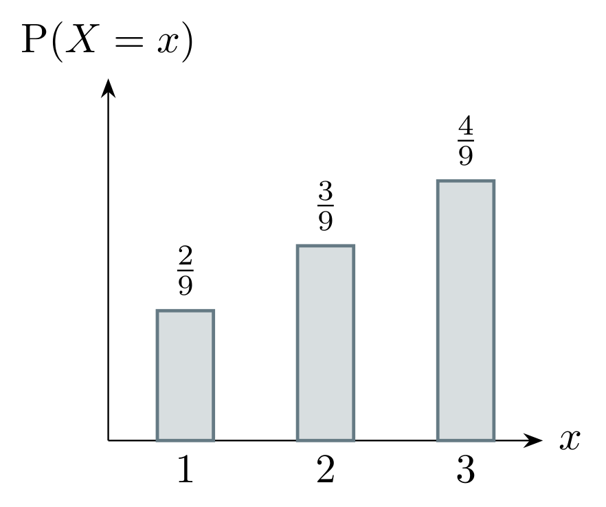
A spinner has three unequal sectors labelled 1, 2 and 3. Let \(X\) be the number obtained on one spin. Its probability distribution is \[\operatorname{P}(X=x)=k(x+1),\qquad x\in\{1,2,3\},\] with probability zero for all other values. Find \(k\) and represent the distribution as a table and a probability bar chart.
Solution
First substitute the allowed values: \[\begin{aligned} \operatorname{P}(X=1)&=k(1+1)=2k,\\ \operatorname{P}(X=2)&=k(2+1)=3k,\\ \operatorname{P}(X=3)&=k(3+1)=4k. \end{aligned}\] Now make the total probability equal to 1: \[2k+3k+4k=1\quad\Longrightarrow\quad 9k=1\quad\Longrightarrow\quad k=\boxed{\frac19}.\]
| \(x\) | \(1\) | \(2\) | \(3\) |
|---|---|---|---|
| \(\operatorname{P}(X=x)\) | \(\frac29\) | \(\frac39\) | \(\frac49\) |
All entries lie between 0 and 1, and \(\frac29+\frac39+\frac49=1\).
How to read a probability bar chart
The horizontal axis shows the possible values of \(X\). The height of the bar above \(x\) is \(\operatorname{P}(X=x)\). To find the probability of several values, add their bar heights.
Use separate bars: values between them are not automatically possible. The vertical axis shows probability, not the number of observations. The bar widths do not encode probability.
Quick check B
For the distribution in example 3, find \(\operatorname{P}(X=2)\) and \(\operatorname{P}(X=2.5)\).
Show solutionHide solution
Solution
\(\operatorname{P}(X=2)=\frac39=\frac13\); \(\operatorname{P}(X=2.5)=0\) because 2.5 is not an allowed value.
Related tutorial: Distribution tables and bar charts
Connect a discrete random variable with its table and graphical representation.
Find probabilities from a distribution
An event is a condition on the outcome. For example, \(X\geq2\) means that the value of \(X\) is at least 2. List the allowed values satisfying the condition, then add their probabilities.
| Wording | Condition | Wording | Condition |
|---|---|---|---|
| Exactly \(a\) | \(X=a\) | More than \(a\) | \(X>a\) |
| At most \(a\) | \(X\le a\) | At least \(a\) | \(X\ge a\) |
| Fewer than \(a\) | \(X<a\) | From \(a\) to \(b\), inclusive | \(a\le X\le b\) |
The complement can save work
The complement of an event is the event that it does not happen. Their probabilities add to 1. For example, \[\boxed{\operatorname{P}(X\leq a)=1-\operatorname{P}(X>a)}.\] Keep the endpoints correct: the complement of “at most \(a\)” is “more than \(a\)”.
Worked example 4 Inequalities and impossible values
Let \(X\) be the change in a player’s score, in points, after one round:
| \(x\) | \(-2\) | \(0\) | \(1\) | \(3\) |
|---|---|---|---|---|
| \(\operatorname{P}(X=x)\) | \(\frac1{10}\) | \(\frac2{10}\) | \(\frac4{10}\) | \(\frac3{10}\) |
Find:
\(\operatorname{P}(X>1)\);
\(\operatorname{P}(X\geq1)\);
\(\operatorname{P}(X\leq0)\) using the complement;
\(\operatorname{P}(X=2)\).
Solution
Only 3 is greater than 1: \(\operatorname{P}(X>1)=\operatorname{P}(X=3)=\boxed{\frac3{10}}\).
Both 1 and 3 are at least 1: \[\operatorname{P}(X\geq1)=\frac4{10}+\frac3{10}=\boxed{\frac7{10}}.\]
The positive values are 1 and 3, so \[\operatorname{P}(X\leq0)=1-\operatorname{P}(X>0)=1-\left(\frac4{10}+\frac3{10}\right)=\boxed{\frac3{10}}.\]
The value 2 is not in the distribution: \(\boxed{\operatorname{P}(X=2)=0}\).
Endpoints can change a discrete probability
Here \(\operatorname{P}(X>1)\ne\operatorname{P}(X\geq1)\) because \(\operatorname{P}(X=1)=\frac4{10}\). Always check whether the endpoint is included.
Quick check C
Using the same table, find \(\operatorname{P}(-1<X\leq3)\). List the values you include.
Show solutionHide solution
Solution
Include 0, 1 and 3. Their probabilities give \(\frac2{10}+\frac4{10}+\frac3{10}=\frac9{10}\).
Expected value: the mean of a random variable
What average value should we expect over many repetitions of a random experiment? More likely values should contribute more to that average. This leads to a probability-weighted mean.
Expected value, also called the mean
\[\boxed{\mu=\operatorname{E}(X)=\sum_x x\operatorname{P}(X=x)}.\] Multiply each possible value by its own probability, then add the products. The symbol \(\mu\) (“mu”) denotes the mean; \(\operatorname{E}(X)\) is read as “the expected value of \(X\)”.
The sum includes one term for each allowed value. For three values \(x_1,x_2,x_3\) with probabilities \(p_1,p_2,p_3\), it is \(x_1p_1+x_2p_2+x_3p_3\).
This expected-value formula is provided in the IB AA formula booklet, SL 4.7.
Worked example 5 Calculate and interpret a mean
Let \(X\) be the number of tokens in one randomly selected envelope, with
| \(x\) | \(0\) | \(2\) | \(5\) |
|---|---|---|---|
| \(\operatorname{P}(X=x)\) | \(\frac15\) | \(\frac12\) | \(\frac3{10}\) |
Find \(\operatorname{E}(X)\) and explain what it means.
Solution
Keep each value matched with its probability:
| \(x\) | \(0\) | \(2\) | \(5\) |
|---|---|---|---|
| \(\operatorname{P}(X=x)\) | \(\frac15\) | \(\frac12\) | \(\frac3{10}\) |
| \(x\operatorname{P}(X=x)\) | \(0\left(\frac15\right)=0\) | \(2\left(\frac12\right)=1\) | \(5\left(\frac3{10}\right)=\frac32\) |
Add the products in the bottom row: \[\operatorname{E}(X)=0\left(\frac15\right)+2\left(\frac12\right)+5\left(\frac3{10}\right)=\boxed{\frac52\text{ tokens}}.\] Over many independent selections with this same distribution, the average number of tokens per envelope will tend towards 2.5. For example, counts near 200, 500 and 300 in 1000 selections would give an average near \(2.5\); actual counts fluctuate.
An expected value need not be a possible value
No envelope contains 2.5 tokens. The most likely count is 2 tokens, but the mean is 2.5. The calculation \((0+2+5)/3\) is incorrect here: it ignores the unequal probabilities.
Quick check D
Let \(W\) take values \(0,2,4\) with probabilities \(\frac12,\frac14,\frac14\). Find \(\operatorname{E}(W)\). Can \(W\) equal its mean on a single trial?
Show solutionHide solution
Solution
\(\operatorname{E}(W)=0(\frac12)+2(\frac14)+4(\frac14)=\frac32\). The mean 1.5 is not a possible value of \(W\).
Related tutorial: Mean and mode of a discrete random variable
Use the mean calculation to reinforce this section. The video also revises the mode: the value with greatest probability.
Use and interpret expected value
An expected value has the same units as the random variable. A mean number of customers is measured in customers; a mean gain measured in euros is also in euros.
When the same model applies to each of \(n\) trials, the expected total is \(n\) times the expected value for one trial. This is an average prediction, not a guaranteed total.
Worked example 6 From a daily mean to an expected total
Let \(X\) be the number of express deliveries made by a small shop in one day:
| \(x\) | \(0\) | \(1\) | \(2\) | \(3\) |
|---|---|---|---|---|
| \(\operatorname{P}(X=x)\) | \(0.10\) | \(0.25\) | \(0.40\) | \(0.25\) |
Find and interpret \(\operatorname{E}(X)\).
Find the expected number of express deliveries over 30 days, assuming this model applies each day.
Solution
Multiply the values by their probabilities and add: \[\begin{aligned} \operatorname{E}(X)&=0(0.10)+1(0.25)+2(0.40)+3(0.25)\\ &=\boxed{1.8\text{ deliveries}}. \end{aligned}\] Over many days, the shop averages about 1.8 express deliveries per day. A single day’s count is still a whole number.
The expected total is \(30(1.8)=\boxed{54\text{ deliveries}}\). The actual total could be different.
Worked example 7 Use a given mean to find probabilities
Let \(X\) be the number of points earned in one round of a game:
| \(x\) | \(0\) | \(2\) | \(6\) |
|---|---|---|---|
| \(\operatorname{P}(X=x)\) | \(p\) | \(\frac12\) | \(q\) |
Given that \(\operatorname{E}(X)=\frac52\), find \(p\) and \(q\).
Solution
There are two unknown probabilities, so use two facts: \[\begin{aligned} p+\frac12+q&=1 &&\text{(total probability)},\\ 0p+2\left(\frac12\right)+6q&=\frac52 &&\text{(expected value)}. \end{aligned}\] From the second equation, \[1+6q=\frac52\quad\Longrightarrow\quad6q=\frac32\quad\Longrightarrow\quad q=\frac14.\] Then \(p=1-\frac12-\frac14=\frac14\). The probabilities \(\frac14,\frac12,\frac14\) lie between 0 and 1 and sum to 1. Check the mean: \[0\left(\frac14\right)+2\left(\frac12\right)+6\left(\frac14\right)=\frac52,\] which agrees with the given value.
Quick check E
A score \(S\) takes values \(0,1,3\) with probabilities \(a,\frac12,\frac12-a\). Given that \(\operatorname{E}(S)=1.1\), find \(a\) and check the probabilities.
Show solutionHide solution
Solution
\(\operatorname{E}(S)=0a+1(\frac12)+3(\frac12-a)=2-3a=1.1\), so \(a=0.3\). The probabilities are \(0.3,0.5,0.2\): all are valid and sum to 1.
Fair games: distinguish a prize from a net gain
A player may receive a prize but also pay to take part. To decide whether a game is fair, work with the player’s net gain: the money received minus the money paid.
Define the quantities before calculating
For one play, let \(R\) be the prize money received, in euros. Let the fixed entry fee be \(c\) euros. Let \(G\) be the player’s net gain, in euros. Then \[\boxed{G=R-c}.\] A positive \(G\) is a profit; a negative \(G\) is a loss; \(G=0\) means the player breaks even on that play.
A game is fair in the expected-value sense when \(\boxed{\operatorname{E}(G)=0}\). A positive expected net gain favours the player; a negative one means an expected loss for the player.
Worked example 8 A prize does not tell the whole story
A player pays €2 to select one prize envelope. Let \(R\) be the prize money received, in euros, on this play:
| \(r\) | \(0\) | \(2\) | \(5\) |
|---|---|---|---|
| \(\operatorname{P}(R=r)\) | \(\frac15\) | \(\frac12\) | \(\frac3{10}\) |
Find the expected prize money, \(\operatorname{E}(R)\).
Define the player’s net-gain distribution and find its mean.
Find the probability that the player makes a profit. Is the game fair?
Solution
\(\operatorname{E}(R)=0(\frac15)+2(\frac12)+5(\frac3{10})=\boxed{\text{€}2.50}\).
Let \(G\) be the player’s net gain, in euros, on this play. Since \(G=R-2\), subtract 2 from each prize; the corresponding probabilities stay the same:
\(\text{Prize }r\) \(0\) \(2\) \(5\) \(\text{Net gain }g\) \(-2\) \(0\) \(3\) \(\operatorname{P}(G=g)\) \(\frac15\) \(\frac12\) \(\frac3{10}\) \[\operatorname{E}(G)=(-2)\left(\frac15\right)+0\left(\frac12\right)+3\left(\frac3{10}\right)=\boxed{\text{€}0.50}.\]
A profit requires \(G>0\), which occurs only when the prize is €5: \[\operatorname{P}(G>0)=\boxed{\frac3{10}}.\] The game is not fair: \(\operatorname{E}(G)>0\). The player gains an average of €0.50 per play in the long run, even though a profit occurs on only 30% of plays.
Quick check F
If the entry fee in example 8 becomes €3 but the prizes stay the same, what is the player’s expected net gain per play?
Show solutionHide solution
Solution
The net gains become \(-3,-1,2\), so \(\operatorname{E}(G)=(-3)(\frac15)+(-1)(\frac12)+2(\frac3{10})=-\text{€}0.50\). The player loses €0.50 per play on average.
Find a fair entry fee or an unknown prize
For these questions, first define the player’s net gain on one play. Express its possible values, calculate its expected value and set that expectation equal to zero.
Worked example 9 Find the fair entry fee
In the envelope game, the prize \(R\) is €0, €2 or €5, with probabilities \(\frac15,\frac12,\frac3{10}\). Find the entry fee \(c\) euros that makes the game fair.
Solution
Let \(G\) be the player’s net gain, in euros, on one play. Since \(G=R-c\), its values are \(-c\), \(2-c\) and \(5-c\), with the same probabilities as the prizes. \[\begin{aligned} \operatorname{E}(G)&=(-c)\left(\frac15\right)+(2-c)\left(\frac12\right)+(5-c)\left(\frac3{10}\right)\\ &=\frac52-c\left(\frac15+\frac12+\frac3{10}\right)\\ &=\frac52-c. \end{aligned}\] For fairness, \(\operatorname{E}(G)=0\), so \(\frac52-c=0\) and \(\boxed{c=2.50}\). The fair entry fee is €2.50.
A useful consequence
When the only payment is a fixed entry fee, the fair entry fee equals the expected prize money. The calculation above explains why: the fee is paid on every play, so it is subtracted once from the expected prize.
Worked example 10 Find the prize that makes a game fair
A spinner has eight equal sectors. One sector wins a prize of €\(w\); the other seven pay nothing. It costs €3 to play. Find \(w\) for a fair game.
Solution
Let \(G\) be the player’s net gain, in euros, on one spin. The possible net gains are
| \(g\) | \(w-3\) | \(-3\) |
|---|---|---|
| \(\operatorname{P}(G=g)\) | \(\frac18\) | \(\frac78\) |
Set the expected net gain equal to zero: \[\begin{aligned} (w-3)\left(\frac18\right)+(-3)\left(\frac78\right)&=0,\\ w-3-21&=0,\\ w&=\boxed{24}. \end{aligned}\] The prize must be €24. Check: the net gains are €21 and \(-\text{€}3\), and \(21(\frac18)-3(\frac78)=0\).
Fair does not mean a 50% chance of making a profit
In example 10, the player makes a profit with probability \(\frac18\), but the game is fair. Fairness concerns the average net gain, including the sizes of gains and losses. It does not guarantee breaking even after a few plays.
Quick check G
A player’s net gain is €9 with probability \(0.1\) and \(-\text{€}1\) with probability \(0.9\). Is the game fair? Explain using expected value.
Show solutionHide solution
Solution
\(\operatorname{E}(G)=9(0.1)+(-1)(0.9)=0\). The game is fair in the expected-value sense, although only 10% of plays make a profit.
Practice and worked solutions
Try each question first, then expand its solution to check your reasoning. Give exact values unless a decimal is requested.
1. Identify a discrete random variable
For each situation, state whether the variable is discrete and explain briefly:
the number of text messages received in one hour;
the exact time taken to run 100 m, before any rounding;
the net gain from a game, whose only possible values are \(-\text{€}1.50\), €0 and €2.50.
Show solutionHide solution
Solution
Discrete: the possible counts are \(0,1,2,\ldots\) messages.
Continuous: exact, unrounded time can take any value in an interval.
Discrete: the possible gains form a finite list. Discrete values may be negative or non-integer.
2. Check both conditions
Each list below is proposed as the probabilities of all three distinct values of a random variable. State whether each list is valid and justify your answer.
\(0.20,\;0.35,\;0.55\);
\(-0.10,\;0.50,\;0.60\).
Show solutionHide solution
Solution
Invalid. Each number lies between 0 and 1, but the total is \(0.20+0.35+0.55=1.10\ne1\).
Invalid. The total is 1, but \(-0.10<0\) cannot be a probability.
3. A probability formula
Let \(X\) be the number of vouchers in a randomly selected packet, with \[\operatorname{P}(X=x)=k(4-x),\qquad x\in\{1,2,3\},\] and probability zero otherwise.
Find \(k\) and write the probability distribution as a table.
Find \(\operatorname{P}(X\geq2)\) and \(\operatorname{P}(X=2.5)\).
Find \(\operatorname{E}(X)\).
Show solutionHide solution
Solution
Substituting \(x=1,2,3\) gives probabilities \(3k,2k,k\). Thus \[3k+2k+k=1\quad\Longrightarrow\quad k=\boxed{\frac16}.\]
\(x\) \(1\) \(2\) \(3\) \(\operatorname{P}(X=x)\) \(\frac12\) \(\frac13\) \(\frac16\) All entries are in \([0,1]\), and their sum is 1.
The values 2 and 3 satisfy \(X\geq2\), so \[\operatorname{P}(X\geq2)=\frac13+\frac16=\boxed{\frac12}.\] The value 2.5 is outside the allowed set, so \(\boxed{\operatorname{P}(X=2.5)=0}\).
Multiply each value by its probability and add: \[\operatorname{E}(X)=1\left(\frac12\right)+2\left(\frac13\right)+3\left(\frac16\right) =\frac12+\frac23+\frac12=\boxed{\frac53\text{ vouchers}}.\]
4. Read a probability bar chart
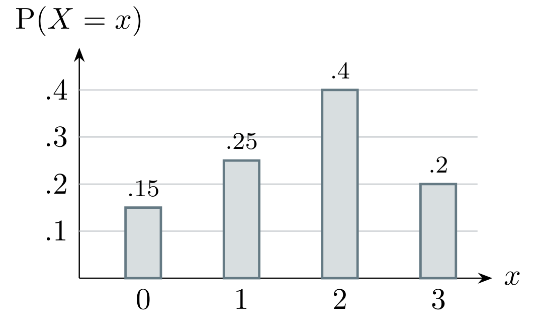
Let \(X\) be the number of items returned to a shop in one hour. Its distribution is shown below.
Write the probability distribution as a table.
Find \(\operatorname{P}(1<X\leq3)\).
Find and interpret \(\operatorname{E}(X)\).
Show solutionHide solution
Solution
Read the height of each bar:
\(x\) \(0\) \(1\) \(2\) \(3\) \(\operatorname{P}(X=x)\) \(0.15\) \(0.25\) \(0.40\) \(0.20\) The allowed values satisfying \(1<X\leq3\) are 2 and 3: \[\operatorname{P}(1<X\leq3)=0.40+0.20=\boxed{0.60}.\]
The probability-weighted mean is \[\operatorname{E}(X)=0(0.15)+1(0.25)+2(0.40)+3(0.20)=\boxed{1.65\text{ items}}.\] Over many hours under this model, the average is about 1.65 returned items per hour.
5. Construct a distribution from an experiment
A bag contains three red counters and one blue counter. A counter is selected at random, replaced, and then a second counter is selected independently. Let \(X\) be the number of blue counters selected in the two draws.
Construct the probability distribution of \(X\).
Find and interpret \(\operatorname{E}(X)\).
Reminder: for independent draws, multiply probabilities along an outcome such as red then blue; add probabilities of different outcomes that give the same count.
Show solutionHide solution
Solution
Because the first counter is replaced, on each draw \(\operatorname{P}(\mathrm B)=\frac14\) and \(\operatorname{P}(\mathrm R)=\frac34\). The outcomes are:
Ordered outcome \(X\) \(\text{Probability}\) Red, red \(0\) \(\frac34\times\frac34=\frac9{16}\) Red, blue \(1\) \(\frac34\times\frac14=\frac3{16}\) Blue, red \(1\) \(\frac14\times\frac34=\frac3{16}\) Blue, blue \(2\) \(\frac14\times\frac14=\frac1{16}\) Combine the two outcomes giving \(X=1\):
\(x\) \(0\) \(1\) \(2\) \(\operatorname{P}(X=x)\) \(\frac9{16}\) \(\frac6{16}\) \(\frac1{16}\) The probabilities sum to 1. Notice that the ordered outcomes are not equally likely in this experiment.
\[\operatorname{E}(X)=0\left(\frac9{16}\right)+1\left(\frac6{16}\right)+2\left(\frac1{16}\right)=\frac8{16}=\boxed{\frac12}.\] Over many repetitions of the two-draw experiment, the mean number of blue counters selected is \(0.5\) per experiment.
6. An expected total
Let \(X\) be the number of customers arriving at a kiosk in a five-minute interval:
| \(x\) | \(0\) | \(1\) | \(2\) | \(3\) | \(4\) |
|---|---|---|---|---|---|
| \(\operatorname{P}(X=x)\) | \(0.10\) | \(0.20\) | \(0.35\) | \(0.25\) | \(0.10\) |
Find and interpret \(\operatorname{E}(X)\).
Assuming this model applies to each interval, find the expected total number of arrivals over 200 such intervals.
Show solutionHide solution
Solution
\[\begin{aligned} \operatorname{E}(X)&=0(0.10)+1(0.20)+2(0.35)+3(0.25)+4(0.10)\\ &=0+0.20+0.70+0.75+0.40\\ &=\boxed{2.05\text{ customers}}. \end{aligned}\] Over many five-minute intervals, the mean arrival count is about 2.05 customers per interval.
Expected total: \(200(2.05)=\boxed{410\text{ customers}}\). This is not a guaranteed count.
7. Two missing probabilities
Let \(X\) be the change in a player’s score, in points, after one round:
| \(x\) | \(-1\) | \(2\) | \(4\) |
|---|---|---|---|
| \(\operatorname{P}(X=x)\) | \(a\) | \(b\) | \(\frac14\) |
Given that \(\operatorname{E}(X)=\frac74\), find \(a\) and \(b\). Verify both the total probability and the given mean.
Show solutionHide solution
Solution
Use total probability and the given mean: \[\begin{aligned} a+b+\frac14&=1 &&\Longrightarrow\quad a+b=\frac34,\\ (-1)a+2b+4\left(\frac14\right)&=\frac74 &&\Longrightarrow\quad -a+2b=\frac34. \end{aligned}\] Adding these equations gives \(3b=\frac32\), so \(\boxed{b=\frac12}\) and \(\boxed{a=\frac14}\).
The probabilities \(\frac14,\frac12,\frac14\) lie between 0 and 1 and sum to 1. The mean is \[(-1)\left(\frac14\right)+2\left(\frac12\right)+4\left(\frac14\right)=-\frac14+1+1=\frac74,\] which agrees with the given value.
8. Fairness and the chance of a profit
Let \(G\) be the player’s net gain, in euros, on one play of a game:
| \(g\) | \(-4\) | \(1\) | \(8\) |
|---|---|---|---|
| \(\operatorname{P}(G=g)\) | \(0.50\) | \(0.35\) | \(0.15\) |
Find and interpret \(\operatorname{E}(G)\).
Find \(\operatorname{P}(G>0)\).
A student says, “The chance of a profit is 50%, so the game is fair.” Explain why this reasoning is incorrect.
Show solutionHide solution
Solution
\(\operatorname{E}(G)=(-4)(0.50)+1(0.35)+8(0.15)=-2+0.35+1.20=\boxed{-\text{€}0.45}\). The player has an expected loss of €0.45 per play.
A profit means \(G>0\): \(\operatorname{P}(G>0)=0.35+0.15=\boxed{0.50}\).
The game is not fair, because \(\operatorname{E}(G)\ne0\). The probability of a profit does not account for the different sizes of gains and losses.
9. Prize money, net gain and a fair fee
A fair six-sided die is rolled once. A player receives €0 for a result from 1 to 4, €6 for a 5 and €12 for a 6. Let \(R\) be the prize received, in euros, on one play.
Write the distribution of \(R\) and calculate \(\operatorname{E}(R)\).
The entry fee is €2. Let \(G\) be the player’s net gain, in euros, on one play. Write its distribution and calculate \(\operatorname{E}(G)\).
Find the entry fee that would make the game fair.
Show solutionHide solution
Solution
Four die results give no prize; one gives €6 and one gives €12:
\(r\) \(0\) \(6\) \(12\) \(\operatorname{P}(R=r)\) \(\frac46\) \(\frac16\) \(\frac16\) \[\operatorname{E}(R)=0\left(\frac46\right)+6\left(\frac16\right)+12\left(\frac16\right)=\boxed{\text{€}3}.\]
With a €2 fee, \(G=R-2\):
\(g\) \(-2\) \(4\) \(10\) \(\operatorname{P}(G=g)\) \(\frac46\) \(\frac16\) \(\frac16\) \[\operatorname{E}(G)=(-2)\left(\frac46\right)+4\left(\frac16\right)+10\left(\frac16\right)=\frac{-8+4+10}{6}=\boxed{\text{€}1}.\]
For a fee of \(c\) euros, the expected net gain is \(3-c\). Set \(3-c=0\) to obtain the fair entry fee of €3.
10. Set a fair prize and interpret the result
A spinner has five equal sectors. One sector pays a prize of €\(w\); the other four pay nothing. A player pays €4 to spin once.
Define the player’s net gain \(G\), state its distribution and find \(w\) so that the game is fair.
Find the probability of a profit when the game is fair.
An alternative gives a guaranteed prize of €4 for the same €4 fee. Compare the two games’ expected net gains and explain one difference between them.
Show solutionHide solution
Solution
Let \(G\) be the player’s net gain, in euros, on one spin. Then
\(g\) \(w-4\) \(-4\) \(\operatorname{P}(G=g)\) \(\frac15\) \(\frac45\) For fairness, \[\begin{aligned} (w-4)\left(\frac15\right)+(-4)\left(\frac45\right)&=0,\\ w-4-16&=0,\\ w&=\boxed{20}. \end{aligned}\] Thus the prize must be €20.
The player makes a profit only on the winning sector, so \(\operatorname{P}(G>0)=\boxed{\frac15}\).
Both expected net gains are €0. The alternative always gives net gain \(4-4=0\). The spinner gives either €16 or \(-\text{€}4\): its individual outcomes vary even though its mean is also zero.
Final review
What you should now be able to do
Define a random variable clearly, including one trial and any units.
Construct or read its table, formula and probability bar chart.
Check that each probability is in \([0,1]\) and that all probabilities sum to 1.
Select the correct values for an event and add their probabilities.
Calculate \(\operatorname{E}(X)=\sum_x x\operatorname{P}(X=x)\) and interpret it as a long-run mean.
Use a known mean and total probability to determine missing probabilities.
Define net gain before using \(\operatorname{E}(G)=0\) to analyse a fair game.
Final checks before you finish a question
Keep values and probabilities in matching order. Preserve negative signs for losses. Include endpoints when required. Keep exact fractions until the final step, and give units and an interpretation for a mean.
For a finite distribution, the mean must lie between its smallest and largest possible values. An answer outside that range signals an error.
Tutorial guide
Use these tutorials alongside the explanations and examples above.
- Distribution tables and bar charts: sections 2–3, connecting the values, probabilities and bar heights. Watch on YouTube.
- Mean and mode of a discrete random variable: section 5, practising the probability-weighted mean. The mode is the most likely value; it need not equal the mean. Watch on YouTube.
Syllabus reference: IB Mathematics: analysis and approaches guide, SL 4.7 (shared SL/HL content), p. 57. Expected-value formula: IB AA formula booklet, SL 4.7. These lesson notes use original worked examples and practice.